Recurrent Networks

Recurrent Networks: With connections allowed both ways between units, and even from a unit to itself.

7.1 Boltzmann Machines(玻尔兹曼机)

Stochastic networks with symmetric connections($w_{ij}=w_{ji}$).

Original form: slow for averaging over stochastic variables.
Mean field version: speeded up and more applications.

Stochastic Units(随机单元)

Visible & hidden units.

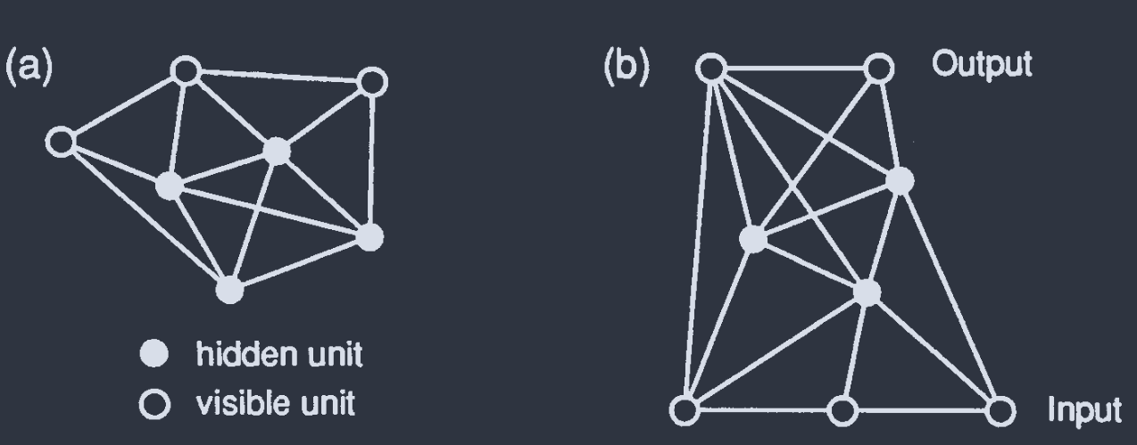
Hidden units: No connection to outside world.

$$ \begin{aligned} P(S_{i} = +1) &= g(h_{i}) = \frac{1}{1+\exp{(-2\beta h_{i})}}\\ P(S_{i} = -1) &= 1 - g(h_{i}) \end{aligned} $$

$\begin{aligned}h_{i} = \sum_{j}w_{ij}S_{j},\quad\beta = 1/T\end{aligned}$.

Energy function:

$$ H(\{S_{i}\}) = -\frac{1}{2}\sum_{ij}w_{ij}S_{i}S_{j},\quad S_{i} = \text{sgn}{(h_{i})} $$

Boltzmann-Gibbs distribution:

$$ P(\{S_{i}\}) = \frac{e^{-\beta H(\{S_{i}\})}}{Z} $$

Partition function: $$Z = \sum_{\{S_{i}\}} e^{-\beta H(\{S_{i}\})}$$

average $\langle X\rangle$:

$$ \langle X\rangle = \sum_{\{S_{i}\}}P(\{S_{i}\}) X(\{S_{i}\}) $$

Pattern completion: At low $T$, only a few possible states have high and equal prob.

$w_{ij}\propto \xi_{i}\xi_{j}$: no information about links with hidden units.

$\alpha$: state of visible units;

$\beta$: state of hidden units.

$N$ visible units, $K$ hidden units $\Rightarrow 2^{N+K}$ possibilities.

Probability $P_{\alpha}$ of chosen state $\alpha$:

$$ \begin{aligned} P_{\alpha} &= \sum_{\beta}P_{\alpha\beta} = \sum_{\beta}\frac{1}{Z}e^{-\beta H_{\alpha\beta}}\\ Z &= \sum_{\alpha\beta}e^{-\beta H_{\alpha\beta}}\\ H_{\alpha\beta} &= -\frac{1}{2}\sum_{ij}w_{ij}S_{i}^{\alpha\beta}S_{j}^{\alpha\beta} \end{aligned} $$

Desired probability: $R_{\alpha}$

Cost function: relative entropy(to measure the difference):

$$ E = \sum_{\alpha}R_{\alpha}\log{\frac{R_{\alpha}}{P_{\alpha}}} = E_{0} {\color{green}{- \sum_{\alpha}R_{\alpha}\log{P_{\alpha}}}}\geq 0 $$

$E = 0$ only if $P_{\alpha} = R_{\alpha}$, $\forall \alpha$.

Gradient descent:

$$ \begin{aligned} {\color{blue}{\Delta w_{ij}}} &= -\eta \frac{\partial E}{\partial w_{ij}} = \eta\sum_{\alpha}\frac{R_{\alpha}}{P_{\alpha}}{\color{red}{\frac{\partial P_{\alpha}}{\partial w_{ij}}}}\\ {\color{red}{\frac{\partial P_{\alpha}}{\partial w_{ij}}}} &= \sum_{\beta}\frac{1}{Z}e^{-\beta H_{\alpha\beta}}S_{i}^{\alpha\beta}S_{j}^{\alpha\beta} - \frac{1}{Z^{2}}\left(\sum_{\beta}e^{-\beta H_{\alpha\beta}}\right)\sum_{\lambda\mu}e^{-\beta H_{\lambda\mu}}S_{i}^{\lambda\mu}S_{j}^{\lambda\mu}\\ &= \beta\left[ \sum_{\beta}S_{i}^{\alpha\beta}S_{j}^{\alpha\beta}P_{\alpha\beta} - P_{\alpha}\langle S_{i}S_{j}\rangle \right]\\ {\color{blue}{\Delta w_{ij}}} &= \eta\beta\left[ \sum_{\alpha}\frac{R_{\alpha}}{P_{\alpha}}\sum_{\beta}S_{i}^{\alpha\beta}S_{j}^{\alpha\beta}P_{\alpha\beta} - \sum_{\alpha}R_{\alpha}\langle S_{i}S_{j}\rangle \right]\\ &= \eta\beta\left[ \sum_{\alpha\beta}R_{\alpha}P_{\beta|\alpha}S_{i}^{\alpha\beta}S_{j}^{\alpha\beta} - \langle S_{i}S_{j}\rangle \right]\\ &= \eta\beta\left[ \overset{\text{Hebb term}}{\overline{\langle S_{i}S_{j}\rangle}_{\text{clamped}}} - \overset{\text{unlearning term}}{\langle S_{i}S_{j}\rangle_{\text{free}}} \right],\quad\text{Boltzmann learning rule} \end{aligned} $$

conditional probability: $P_{\beta|\alpha} = P_{\alpha\beta}/P_{\alpha}$.

$\overline{\langle S_{i}S_{j}\rangle}_{\text{clamped}}$: 在给定 $\alpha$ 概率为 $R_{\alpha}$ 的条件下, $S_{i}S_{j}$ 的平均值

Bring the system to equilibrium before taking an average.

Monte Carlo simulation:

Two kinds of methods:

Select a unit at random, update its state according to $P(S_{i} = \pm 1)$.
Flip a unit with prob $$P(S_{i}\rightarrow -S_{i}) = \frac{1}{1+\exp{(\beta\Delta H_{i})}}.$$ Slow at low $T$ (tends to get trapped in local minima)

Faster solution: simulated annealing procedure(渐进模拟)

Adjust weights for convergence;
Calculate $\langle S_{i}S_{j}\rangle$ in clamped and freestates;
Annealing schedule $T(t)$;
Sample and update units.

Fast simulated annealing(Cauchy machine): multiple flips.

Slow but effective.

Variations on Boltzmann Machines(玻尔兹曼机的变种)

Weight decay terms $w_{ij}^{\text{new}} = (1-\varepsilon)w_{ij}^{\text{old}}$: automatically become symmetric;
Incremental rule(增量规则)

If $S_{i}$ & $S_{j}$ on together, step size $\varepsilon$, clamped: $w_{ij}\uparrow$; free: $w_{ij}\downarrow$

Avoid oscillations in valley when relying on local gradient

$\exist \alpha$, $R_{\alpha}=0$. increase it to $\epsilon>0$ to avoid infinite weights.

Input($\gamma$), output($\alpha$), hidden($\beta$). Learn $\gamma\rightarrow \alpha$ (即目标是令 $P_{\alpha|\gamma}=R_{\alpha|\gamma}$)

Error measure(entropic cost function):

$$ E = \sum_{\gamma}p_{\gamma}\sum_{\alpha}R_{\alpha|\gamma}\log{\frac{R_{\alpha|\gamma}}{P_{\alpha|\gamma}}} $$

Learning rule:

$$ \Delta w_{ij} = \eta\beta\left[ \overline{\langle S_{i}S_{j}\rangle}_{\text{I,O clamped}} - \overline{\langle S_{i}S_{j}\rangle}_{\text{I clamped}} \right] $$

Harmonium: two-layer Boltzmann machine. Connections between layers only.
Hopfield: without hidden units. Average $\xi_{i}^{\mu}\xi_{j}^{\mu}$ over patterns $\mu$. Start from random cfg and relax at $T=0$. Faster than incremental one.

Statistical Mechanics Reformulation(统计力学重构)

$P_{\alpha}$: Prob of visible units in state $\alpha$

$\begin{aligned}Z_{\text{clamped}}^{\alpha} = \sum_{\beta}e^{-\beta H_{\alpha\beta}}\end{aligned}$: Partition function (visible units clamped in state $\alpha$)

$$ Z = e^{-\beta F} $$

$$ P_{\alpha} = \frac{Z_{\text{clamped}}^{\alpha}}{Z} = \frac{e^{-\beta F_{\text{clamped}}^{\alpha}}}{e^{-\beta F}} = e^{-\beta (F_{\text{clamped}}^{\alpha} - F)} $$

Cost function:

$$ \begin{aligned} E = E_{0} - \sum_{\alpha}R_{\alpha}\log{P_{\alpha}} &= E_{0} + \beta\sum_{\alpha}R_{\alpha}(F_{\text{clamped}}^{\alpha} - F)\\ &= E_{0} + \beta\left[ \overline{F_{\text{clamped}}^{\alpha}} - F \right] \end{aligned} $$

$$ \begin{aligned} \langle S_{i}S_{j}\rangle &= -\frac{\partial F}{\partial w_{ij}} \\ &= T\frac{\partial \log{Z}}{\partial w_{ij}} = \frac{T}{Z}\frac{\partial Z}{\partial w_{ij}} = \frac{1}{Z}\sum_{\alpha\beta} S_{i}^{\alpha\beta}S_{j}^{\alpha\beta}e^{-\beta H_{\alpha\beta}} \end{aligned} $$

Deterministic Boltzmann Machines(确定性玻尔兹曼机)

Mean field annealing: $\begin{aligned}m_{i}\equiv\langle S_{i}\rangle = \tanh{\left(\beta\sum_{j}w_{ij}m_{j}\right)},\quad \langle S_{i}S_{j}\rangle\approx m_{i}m_{j}\end{aligned}$

Iteration

$$ m_{i}^{\text{new}} = \tanh{\left(\beta\sum_{j}w_{ij}m_{j}^{\text{old}}\right)} $$

Entropy:

$$ S = - \sum_{i}\left( p_{i}^{+}\log{p_{i}^{+}} + p_{i}^{-}\log{p_{i}^{-}} \right), \quad p_{i}^{\pm} = P(S_{i} = \pm 1) $$

$p_{i}^{+} + p_{i}^{-} = 1$, $m_{i} = p_{i}^{+} - p_{i}^{-}$

$$ p_{i}^{\pm} = \frac{1\pm m_{i}}{2} $$

Mean field free energy:

$$ \begin{aligned} F_{\text{MF}} &= H - TS \\ &= -\frac{1}{2}\sum_{ij}w_{ij}m_{i}m_{j} + T\sum_{i}\left( \frac{1+m_{i}}{2}\log{\frac{1+m_{i}}{2}} + \frac{1-m_{i}}{2}\log{\frac{1-m_{i}}{2}} \right) \end{aligned} $$

$$ E = E_{0} + \beta\left[ \overline{F_{\text{clamped}}^{\alpha}} - F \right]\overset{\text{MF}}{\longrightarrow}E_{\text{MF}} = E_{0} + \beta\left[ \overline{F_{\text{MF}}^{\alpha}} - F_{\text{MF}} \right] $$

Gradient descent for $w_{ij}$:

$$ \Delta w_{ij} = -\eta\frac{\partial E_{\text{MF}}}{\partial w_{ij}} = \eta\beta \bigg[\overline{m_{i}^{\alpha}m_{i}^{\alpha}} - m_{i}m_{j}\bigg] $$

原型: $$ \Delta w_{ij} = \eta\beta \bigg[\overline{\langle S_{i}S_{j}\rangle}_{\text{clamped}} - \langle S_{i}S_{j}\rangle_{\text{free}}\bigg] $$

7.2 Recurrent Back-Propagation(递归反向传播)

$V_{i}$: $N$ continuous-valued units

$w_{ij}$: connections

$g(h)$: activation function

$\zeta_{i}^{\mu}$: desired training values.

Dynamic evolution rules:

$$ \tau\frac{\mathrm{d}V_{i}}{\mathrm{d}t} = -V_{i} + g\left( \sum_{j}w_{ij}V_{j} + \xi_{i} \right) $$

fixed point equation $\begin{aligned}\left(\frac{\mathrm{d}V_{i}}{\mathrm{d}t} = 0\right)\end{aligned}$:

$$ V_{i} = g(h_{i}) = g\left( \sum_{j}w_{ij}V_{j} + \xi_{i} \right) $$

Assumption: At least 1 fixed point exists and is a stable attractor.

Error measure(Cost function):

$$ E = \frac{1}{2}\sum_{k}E_{k}^{2},\quad E_{k} = \begin{cases} \zeta_{k} - V_{k} & \text{if }k\text{ is output unit}\\ 0 & \text{otherwise} \end{cases} $$

Gradient descent:

$$ \Delta w_{pq} = -\eta\frac{\partial E}{\partial w_{pq}} = \eta\sum_{k}E_{k}\frac{\partial V_{k}}{\partial w_{pq}} $$

Differentiating fixed point equation:

$$ \begin{aligned} \frac{\partial V_{i}}{\partial w_{pq}} &= g^{\prime}(h_{i}){\color{red}{\frac{\partial h_{i}}{\partial w_{pq}}}}\\ {\color{red}{\frac{\partial h_{i}}{\partial w_{pq}}}} &= \frac{\partial }{\partial w_{pq}}\left(\sum_{j}{\color{blue}{w_{ij}V_{j}}} + \xi_{i}\right)\\ \frac{\partial ({\color{blue}{w_{ij}V_{j}}})}{\partial w_{pq}} &= {\color{green}{\frac{\partial w_{ij}}{\partial w_{pq}}}}V_{j} + w_{ij}\frac{\partial V_{j}}{\partial w_{pq}} = {\color{green}{\delta_{ip}\delta_{jq}}}V_{j} + w_{ij}\frac{\partial V_{j}}{\partial w_{pq}}\\ \Rightarrow {\color{red}{\frac{\partial h_{i}}{\partial w_{pq}}}} &= \sum_{{\color{green}{j}}}\left( \delta_{ip}\delta_{{\color{green}{j}}q}V_{{\color{green}{j}}} + w_{ij}\frac{\partial V_{j}}{\partial w_{pq}} \right) = \delta_{ip}V_{q} + \sum_{j}w_{ij}\frac{\partial V_{j}}{\partial w_{pq}}\\ \Rightarrow \frac{\partial V_{i}}{\partial w_{pq}} &= g^{\prime}(h_{i})\left( \delta_{ip}V_{q} + \sum_{j}w_{ij}\frac{\partial V_{j}}{\partial w_{pq}} \right)\\ &= \delta_{ip}g^{\prime}(h_{i})V_{q} + \sum_{j}g^{\prime}(h_{i})w_{ij}\frac{\partial V_{j}}{\partial w_{pq}} \end{aligned} $$

将单项写作 delta-求和形式 $\begin{aligned}\frac{\partial V_{i}}{\partial w_{pq}} = \sum_{j}\delta_{ij}\frac{\partial V_{j}}{\partial w_{pq}}\end{aligned}$, 再将等式右边第二项移到左边

$$ \sum_{j}{\color{red}{\bigg[\delta_{ij}-g^{\prime}(h_{i})w_{ij}\bigg]}}\frac{\partial V_{j}}{\partial w_{pq}} = \delta_{ip}g^{\prime}(h_{i})V_{q}\\ \sum_{j}{\color{red}{\mathbf{L}_{ij}}}\frac{\partial V_{j}}{\partial w_{pq}} = \delta_{ip}g^{\prime}(h_{i})V_{q} $$

实际可以理解为 $\mathbf{L}_{i\times j}\times \frac{\partial \mathbf{V}}{\partial w_{pq}}_{j\times 1}$ 的矩阵乘法. 左右同时左乘 $\mathbf{L}^{-1}$:

$$ \frac{\partial V_{k}}{\partial w_{pq}} = (\mathbf{L}^{-1})_{kp}g^{\prime}(h_{p})V_{q} $$

delta-rule:

$$ \begin{aligned} \Delta w_{pq} &= \eta{\color{red}{\sum_{k} E_{k}(\mathbf{L}^{-1})_{kp}g^{\prime}(h_{p})}}V_{q}\\ &= \eta{\color{red}{\delta_{p}}}V_{q} \end{aligned} $$

Recall: delta rule 是源自梯度下降的概念, 但是可以被推广为更普适的形式.

Cost function:

$$ E[\vec{w}] = \frac{1}{2}\sum_{i\mu}(\zeta_{i}^{\mu} - O_{i}^{\mu})^{2} = \frac{1}{2}\sum_{i\mu}\left(\zeta_{i}^{\mu}-\sum_{k}w_{ik}\xi_{k}^{\mu}\right)^{2} $$

$$ \Delta w_{ik} = -\eta\frac{\partial E}{\partial w_{ik}} = \eta\sum_{\mu}(\zeta_{i}^{\mu} - O_{i}^{\mu})\xi_{k}^{\mu} $$

对于某固定 $\mu$:

$$ \Delta w_{ik} = \eta(\zeta_{i}^{\mu}-O_{i}^{\mu})\xi_{k}^{\mu} = {\color{red}{\eta\delta_{i}\xi_{k}^{\mu}}} $$

需要求逆而耗费时间.

改进:

$$ \delta_{p} = {\color{red}{\sum_{k} E_{k}(\mathbf{L}^{-1})_{kp}}}g^{\prime}(h_{p}) = g^{\prime}(h_{p}){\color{red}{Y_{p}}} $$

$$ \begin{aligned} \sum_{p}\mathbf{L}_{pi}Y_{p} &= \sum_{p}\mathbf{L}_{pi}\left[ \sum_{k}E_{k}(\mathbf{L}^{-1})_{kp} \right] \\ &= \sum_{k}E_{k}\left[ \sum_{p}\mathbf{L}_{pi}(\mathbf{L}^{-1})_{kp} \right]\\ &= \sum_{k}E_{k}\delta_{ik} = E_{i} \end{aligned} $$

Recall: $$ \mathbf{L}_{ij} = \delta_{ij} - g^{\prime}(h_{i})w_{ij} $$

那么

$$ \begin{aligned} \sum_{p}\mathbf{L}_{pi}Y_{p} &= \sum_{p}\bigg[ \delta_{pi}-g^{\prime}(h_{p})w_{pi} \bigg]Y_{p} \\ &= \sum_{p}\delta_{pi}Y_{p} - \sum_{p}g^{\prime}(h_{p})w_{pi}Y_{p} \\ &= \boxed{Y_{i} - \sum_{p}g^{\prime}(h_{p})w_{pi}Y_{p} = E_{i}} \end{aligned} $$

Error-propagation network:

$$ \tau\frac{\mathrm{d}Y_{i}}{\mathrm{d}t} = - Y_{i} + \sum_{p}g^{\prime}(h_{p})w_{pi}Y_{p} + E_{i} $$

$w_{ij}\rightarrow g^{\prime}(h_{i})w_{ij}$

$g(x)\rightarrow x$

network transposition(网络转置): 通过转置避免显式求逆

Procedure:

$\begin{aligned}\tau\frac{\mathrm{d}V_{i}}{\mathrm{d}t} = -V_{i} + g\left(\sum_{j}w_{ij}V_{j} + \xi_{i}\right)\end{aligned}$ 以找到 $V_{i}$;
$\begin{aligned}E_{k} = \begin{cases}\zeta_{k}-V_{k} & k\text{ is output}\\0&\text{ others}\end{cases}\end{aligned}$ 以确定 $E_{i}$;
$\begin{aligned}\tau\frac{\mathrm{d}Y_{i}}{\mathrm{d}t} = - Y_{i} + \sum_{p}g^{\prime}(h_{p})w_{pi}Y_{p} + E_{i}\end{aligned}$ 以找到 $Y_{i}$;
$\Delta w_{pq}=\eta\delta_{p}V_{q}$, $\delta_{p} = g^{\prime}(h_{p})Y_{p}$ 更新权重.

without requiring any non-local operations(matrix inversion)

original network: supply error signals $E_{i}$;

error-propagation network: adjust weights in the original network.

$\begin{aligned}Y_{i} - \sum_{p}g^{\prime}(h_{p})w_{pi}Y_{p} = E_{i}\end{aligned}$ is a stable attractor if $\begin{aligned}V_{i} = g\left(\sum_{j}w_{ij}V_{j} + \xi_{i}\right)\end{aligned}$ is a stable attractor.

设 $V_{i}^{*}$ 和 $Y_{i}^{*}$ 各为两个动力学方程的不动点. 研究其邻域 $V_{i} = V_{i}^{*} + \epsilon_{i}$ 和 $Y_{i} = Y_{i}^{*} + \eta_{i}$. 代入微分方程且保留一阶项:

$$ \begin{aligned} \tau\frac{\mathrm{d}\epsilon_{i}}{\mathrm{d}t} &= -\epsilon_{i} + g^{\prime}(h_{i})\sum_{j}w_{ij}\epsilon_{j} = -\sum_{j}\mathbf{L}_{ij}\epsilon_{j}\\ \tau\frac{\mathrm{d}\eta_{i}}{\mathrm{d}t} &= -\eta_{i} + \sum_{p}g^{\prime}(h_{p})w_{pi}\eta_{p} = -\sum_{p}\mathbf{L}_{ip}^{T}\eta_{p} \end{aligned} $$

$\mathbf{L}$ 和 $\mathbf{L}^{T}$ 特征值相同, 所以局部稳定性一致.

全连接网络($\mathbf{L}_{N\times N}$)求逆时间复杂度为 $\mathcal{O}(N^3)$. 而网络转置法的时间复杂度为 $\mathcal{O}(N^2)$.

7.3 Learning Time Sequences(时间序列学习)

Sequence Recognition(序列识别): specific input sequence $\to$ particular output pattern
Sequence Reproduction(序列再现): generate the rest of a sequence given part of it.
Temporal Association(时间关联): particular output sequence in response to a specific input sequence.

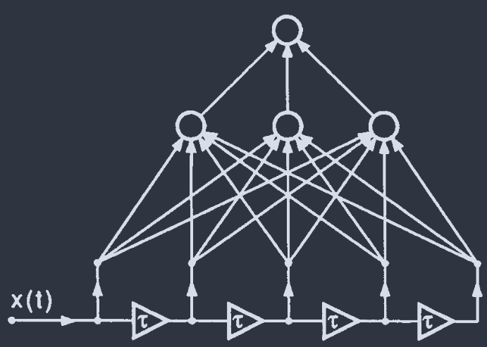
Tapped Delay Lines(抽头延迟线)

time-delay neural networks:

从信号 $x[t]$ 中采集的 $x[\tau], x[\tau-\Delta], \cdots, x[\tau-(m-1)\Delta]$ 同时作为网络输入.

not for arbitrary-length sequences, 不灵活;
large training examples, slow computation, 耗算力;
precise clock, 同步要求高.

Tank & Hopfield:

设 raw signal $\vec{x}(t)$.

Usual delay line: $\vec{x}(t), \vec{x}(t-\tau_{1}),\vec{x}(t-\tau_{2}),\cdots, \vec{x}(t-\tau_{m})$;
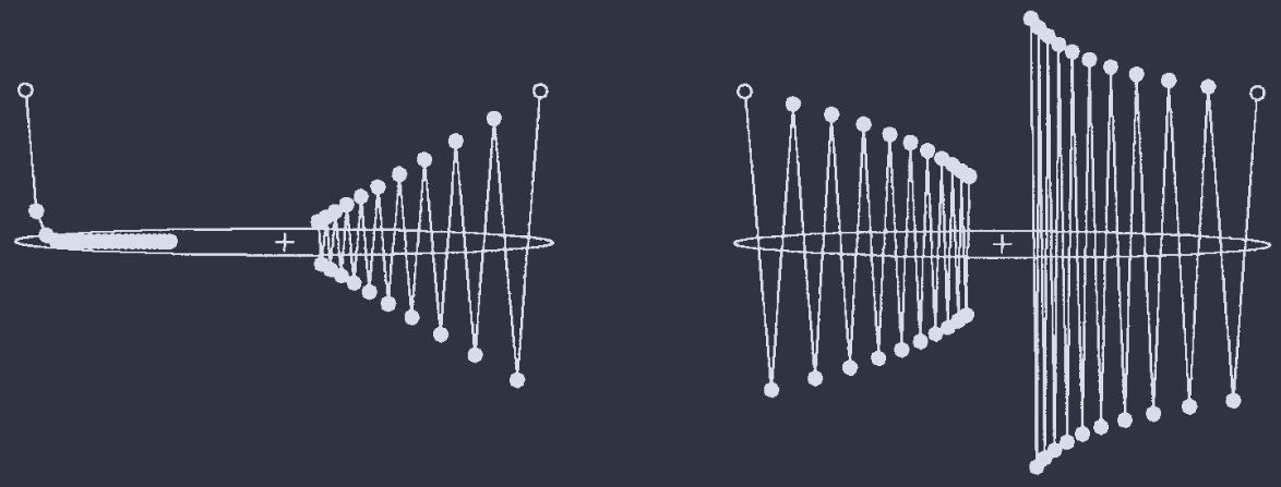
Tank & Hopfield: $\begin{aligned} y(t;\tau_{i}) = \int_{-\infty}^{t}G(t-t^{\prime};\tau_{i})\vec{x}(t^{\prime})\mathrm{d}t^{\prime}\end{aligned}$

$$ G(t;\tau_{i}) = \left(\frac{t}{\tau_{i}}\right)^{\alpha}e^{\alpha(1-t/\tau_{i})} $$

$t=\tau_{i}$ 取极值 1. $\alpha$ 越大 $G$ 越尖锐.

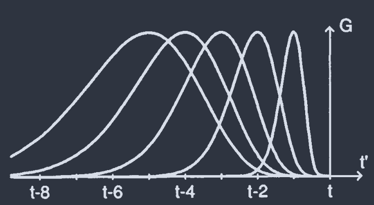
no need for precise synchronization by a central clock.

类似于卷积+滑动窗口(window) 的思路.

Context Units(上下文/记忆单元)

Partially recurrent networks(sequential networks):

mainly feed-forward;
chosen set of feed-back connections

context units $C_{i}$: receive clocked feedback signals.

$t$ 时刻, context unit 接收 $t-1$ 的网络信号

单箭头: 第 $i$ 单元只连接下一层的第 $i$ 单元

阴影箭头: 每一个神经元都和上一层的所有神经元连接

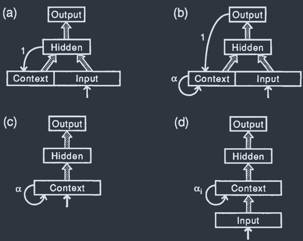
(a) context units hold a copy of the activations of the hidden units from the previous time step.

(b) updating rule:

$$ C_{i}(t+1) = \alpha C_{i}(t) + O_{i}(t) $$

$O_{i}$: output units;

$\alpha < 1$: strength of the self-connections.

If $O_{i}$ fixed: $C_{i}\to O_{i}/(1-\alpha)$

因此, 也被称作 decay/integrating/capacitive units.

Iterating:

$$ \begin{aligned} C_{i}(t+1) &= O_{i}(t) + \alpha O_{i}(t-1) + \alpha^{2}O_{i}(t-2)+\cdots\\ &= \sum_{t^{\prime}=0}^{t}\alpha^{t-t^{\prime}}O_{i}(t^{\prime})\\ &\Rightarrow \int_{0}^{t}e^{-\gamma (t-t^{\prime})}O_{i}(t^{\prime})\mathrm{d}t^{\prime},\quad \gamma = |\log{\alpha}| \end{aligned} $$

这表明 $\alpha$ 应当和输入序列的时间尺度相匹配. 可以使用多个 context 单元组, 每组有不同的 $\alpha$ 值.

(c) Feedback: context units themselves only.

(d)

Input 和 context 之间的连接为全连接而非逐一连接.
Self-connections can be trained.

Back-propagation: No modifiable recurrent connections.

Mozer:

$$ C_{i}(t+1) = \alpha_{i}C_{i}(t) + g\left( \sum_{j}w_{ij}\xi_{j} \right) $$

$\xi_{j}$: input pattern

Williams & Zipser:

$$ C_{i}(t+1) = g\left[ \alpha_{i}C_{i}(t) + \sum_{j}w_{ij}\xi_{j} \right] $$

Back-Propagation Through Time(时间反向传播)

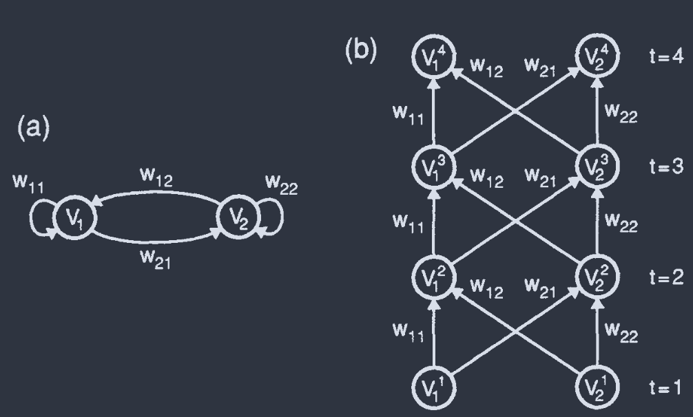
fully recurrent networks: Any unit $V_{i}$ may be connected to any other.

Update rule:

$$ V_{i}(t+1) = g[h_{i}(t)] = g\left[ \sum_{j}w_{ij}V_{j}(t) + \xi_{i}(t) \right] $$

$\xi_{i}(t)$: input at node $i$, at time $t$. 不存在时为 $0$.

Produce $\zeta_{i}(t)$ in response to input sequence $\xi_{i}(t)$

Trick: 任意 recurrent network 可展开为等效 feed-forward network.

2-unit, $T=4$. $w_{ij}$ independent of $t$.

No clock needed;

Need large computer resources:

Storage;
Computer time for simulation;
Number of training examples.

Once trained (in unfolded form), it works for temporal association task.

Real-Time Recurrent Learning(实时递归学习)

Learning rule without duplicating the units.

Deal with sequence of arbitrary length.

Dynamics:

$$ V_{i}(t) = g[h_{i}(t-1)] = g\left[ \sum_{j}w_{ij}V_{j}(t-1) + \xi_{i}(t-1) \right] $$

$\zeta_{k}(t)$: target output

Error measure:

$$ E_{k}(t) = \begin{cases} \zeta_{k}(t) - V_{k}(t) & \text{if }\zeta_{k}(t)\text{ is defined at time }t\\ 0 & \text{otherwise} \end{cases} $$

Cost function:

$$ E = \sum_{t=0}^{T} E(t) $$

$$ E(t) = \frac{1}{2}\sum_{k}[E_{k}(t)]^{2},\quad t = 0,1,2,\cdots,T $$

Gradient descent:

$$ \Delta w_{pq}(t) = -\eta\frac{\partial E(t)}{\partial w_{pq}} = \eta\sum_{k}E_{k}(t)\frac{\partial V_{k}(t)}{\partial w_{pq}} $$

differentiating dynamics:

$$ \frac{\partial V_{i}(t)}{\partial w_{pq}} = g^{\prime}[h_{i}(t-1)]\left[ \delta_{ip}V_{q}(t-1) + \sum_{j}w_{ij}\frac{\partial V_{j}(t-1)}{\partial w_{pq}} \right] $$

Recall: $$ \frac{\partial V_{i}}{\partial w_{pq}} = g^{\prime}(h_{i})\left( \delta_{ip}V_{q} + \sum_{j}w_{ij}\frac{\partial V_{j}}{\partial w_{pq}} \right) $$

If only a stable attractor interested, let $\partial_{w_{pq}}V_{i}(t)=\partial_{w_{pq}}V_{i}(t-1)$, or $\partial_{w_{pq}}V_{i}(0)=0$

$N$ units, $N^{3}$ derivatives($N$ neurons $\times N^{2}$ weights), $\mathcal{O}(N^{4})$ time complexity($N^{3}$ derivatives $\times N$ nodes).

Real-time recurrent learning: Weight update in real time

Avoid array storage.

teacher forcing: always replace $V_{k}(t)$ by $\zeta_{k}(t)$ after $E_{k}(t)$ & derivatives computed.

加速训练收敛, 避免早期预测错误的积累.

Attractor under teacher forcing may be removed when the network runs freely, even turn into a repellor(排斥子)

flip-flop(触发器): if “A $\to$ (arbitrary interval) $\to$ B”: output a signal.

Tapped delay line could never do this.

Time-Dependent Recurrent Back-Propagation(含时递归反向传播)

dynamics:

$$ \tau_{i}\frac{\mathrm{d}V_{i}}{\mathrm{d}t} = -V_{i} + g\left( \sum_{j}w_{ij}V_{j} \right) + \xi_{i}(t)\tag{*} $$

Recall: Recurrent Back-Propagation $$ \tau\frac{\mathrm{d}V_{i}}{\mathrm{d}t} = -V_{i} + g\left(\sum_{j}w_{ij}V_{j} + \xi_{i}\right) $$

Error function:

$$ E = \frac{1}{2}\int_{0}^{T}\sum_{k\in O}[V_{k}(t)-\zeta_{k}(t)]^{2}\mathrm{d}t $$

$O$: output units

$\zeta_{k}(t)$: target output

Gradient descent:

functional derivative(泛函导数):

$$ E_{k}(t) = \frac{\delta E}{\delta V_{k}(t)} = [V_{k}(t) - \zeta_{k}(t)] $$

gradient:

$$ \frac{\partial E}{\partial w_{ij}} = \frac{1}{\tau_{i}}\int_{0}^{T}Y_{i}g^{\prime}(h_{i})V_{j}\mathrm{d}t $$

可以通过 $\begin{aligned}\frac{\partial E}{\partial \tau_{i}}\end{aligned}$ 从而通过调整 $\tau_{i}$ 进行优化.

$\begin{aligned}h_{i}(t) = \sum_{j}w_{ij}V_{j}(t)\end{aligned}$

$Y_{i}(t)$: solution of

$$ \frac{\mathrm{d}Y_{i}}{\mathrm{d}t} = \frac{1}{\tau_{i}}Y_{i} - \sum_{j}\frac{1}{\tau_{j}}w_{ji}g^{\prime}(h_{j})Y_{j} - E_{i}(t),\quad Y_{i}(T) = 0, \forall i\tag{**} $$

recall:

$$ \mathbf{L}_{ij} = \delta_{ij} - g^{\prime}(h_{i})w_{ij}\\ Y_{p} = \sum_{k}E_{k}(\mathbf{L}^{-1})_{kp} $$ error propagation network dynamics: $$ \tau\frac{\mathrm{d}Y_{i}}{\mathrm{d}t} = -Y_{i} + \sum_{p}g^{\prime}(h_{p})w_{pi}Y_{p} + E_{i} $$

$\int_{0}^{T}(*)\Rightarrow V_{i}(t)$;

$\int_{T}^{0}(**)\Rightarrow Y_{i}(t)$.

so that we get $\begin{aligned}\Delta w_{ij} = -\eta\frac{\partial E}{\partial w_{ij}}\end{aligned}$

large time & storage requirements: $N$ fully recurrent units & $K$ time steps ($0\to T$)

time per forward-backward pass $\sim N^{2}K$ (Real-Time Recurrent Learning: $\sim N^{4}K$)
memory $\sim aNK+bN^{2}$ (RTRL: $\sim N^{3}$)

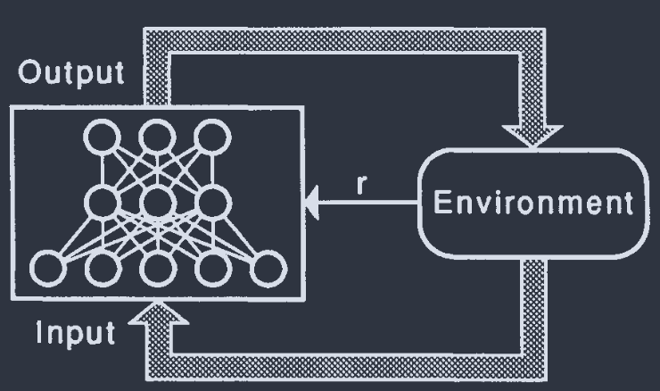
7.4 Reinforcement Learning(强化学习)

No detailed target values. Only “right” or “wrong”. Learn with a critic, not a teacher.

Introduce randomness to explore a correct value(by using stochastic units).

Reinforcement learning problems:

I. Same signal for a given i-o pair. (IO mapping) No reference to previous outputs.
II. Stochastic environment. Given same io-pair, fixed probability distribution of reinforcement. Independent of history.

Two-armed bandit problem(双臂赌博): 两个未知概率的老虎机. 找到平均收益最高的一个. Method: stochastic learning automata(随机学习自动机)

III. Reinforcement & input patterns depend on the output history arbitrarily. Game theory(博弈论): “environment” = other players.

[Example] Chess. Win/lose after a long sequence of moves. Credit assignment problem: how to judge each move’s contribution to victory/defeat?

Associative Reward-Penalty(联想奖惩) $A_{\text{RP}}$

$S_{i}=\pm 1$: output units

Dynamical rule:

$$ P(S_{i} = \pm 1) = g(\pm h_{i}) = f_{\beta}(\pm h_{i}) = \frac{1}{1+\exp{(\mp 2\beta h_{i})}} $$

$$ h_{i} = \sum_{j}w_{ij}V_{j} $$

$V_{j}$: activations of hidden/input units.

Reinforcement signal $r=\pm 1$ (reward/penalty).

Target patterns:

$$ \zeta_{i}^{\mu} = \begin{cases} +S_{i}^{\mu} & \text{if }r^{\mu} = +1\\ -S_{i}^{\mu} & \text{if }r^{\mu} = -1 \end{cases} $$

Recall: Stochastic Units

$$ \begin{aligned} P(S_{i}=\pm 1) &= f_{\beta}(\pm h_{i}) = \frac{1}{1+\exp{(\mp 2\beta h_{i})}},\quad h_{i}^{\mu} = \sum_{k}w_{ik}\xi_{k}^{\mu}\\ \langle S_{i}^{\mu}\rangle &= (+1)g(h_{i}^{\mu}) + (-1)[1-g(h_{i}^{\mu})] = \tanh{\left(\beta h_{i}^{\mu}\right)}\\ \Delta w_{ik} &= \eta\delta_{i}^{\mu}\xi_{k}^{\mu}, \quad \delta_{i}^{\mu} = \zeta_{i}^{\mu} - \langle S_{i}^{\mu}\rangle \end{aligned} $$

Weight update rule

$$ \Delta w_{ij} = \eta(r^{\mu})\delta_{i}^{\mu}V_{j}^{\mu} $$

$\times g^{\prime}(h_{i}^{\mu})$ to minimize $\begin{aligned}\sum_{i}(\delta_{i}^{\mu})^{2}\end{aligned}$ (not for entropic cost function).

$\eta(+1)$ is 10-100 times larger than $\eta(-1)$

So the learning rule

$$ \Delta w_{ij} = \begin{cases} \eta^{+}[+S_{i}^{\mu}-\langle S_{i}^{\mu}\rangle]V_{j}^{\mu} & \text{if }r^{\mu} = +1\\ \eta^{-}[-S_{i}^{\mu}-\langle S_{i}^{\mu}\rangle]V_{j}^{\mu} & \text{if }r^{\mu} = -1 \end{cases} $$

$\eta^{\pm 1} = \eta(\pm 1)$.

Slow compared to supervised learning. Speed depends on the size of the output space and correct fraction of it.

[Example] Only 1 correct answer for each input, the search can be very long.

Variations on $A_{\text{RP}}$:

0/1 units. $-S_{i}^{\mu}\to 1-S_{i}^{\mu}$, $\langle S_{i}^{\mu}\rangle\to p_{i}^{\mu}$.
continuous-valued reward $r\in [0,1]$ for $[\text{terrible}, \text{excellent}]$. simplify the formula:

$$ \Delta w_{ij} = \eta(r^{\mu})\{ r^{\mu}[S_{i}^{\mu} - \langle S_{i}^{\mu}\rangle] + (1-r^{\mu})[-S_{i}^{\mu} - \langle S_{i}^{\mu}\rangle] \}V_{j}^{\mu} $$

for penalty case, use $\langle S_{i}^{\mu}\rangle - S_{i}^{\mu}$ instead of $-S_{i}^{\mu} - \langle S_{i}^{\mu}\rangle$:

$$ \Delta w_{ij} = \eta r^{\mu}[S_{i}^{\mu}-\langle S_{i}^{\mu}\rangle]V_{j}^{\mu} $$

ignore dependence of $\eta$ on $r$.

$r=-1$. 标准形式: 和目前所做相反; 此形式: 不要做目前所做.

standard form works better for larger weight changes.

this variation is more amenable to theoretical analysis.

speed $\uparrow$: present $\mu$ several times before moving to the next pattern. batch mode: accumulating all $\Delta w$

Theory of Associative Reward-Penalty(联想奖惩理论)

Convergence: proved only in special cases.

Usual approach: Cost function $\to \epsilon$

Not so satisfactory for the stochastic process.

Cost function: $-\langle r\rangle$

$E\downarrow \Rightarrow \langle r\rangle\uparrow$

$V_{j}\to \xi_{j}$. Deterministic environment(class I). So $r = r(\mathbf{S},\mathbf{\xi})$

$\mathbf{S}$: output pattern; $\mathbf{\xi}$: input pattern.

$$ \langle r^{\mu}\rangle = \sum_{\mathbf{S}}P(\mathbf{S}|\mathbf{w},\xi^{\mu})r(\mathbf{S},\xi^{\mu}) $$

$P(\mathbf{S}|\mathbf{w},\mathbf{\xi}^{\mu})$: prob of $\mathbf{S}$ if $\mathbf{w}$ and $\mathbf{\xi}^{\mu}$.

$$ P(\mathbf{S}|\mathbf{w},\mathbf{\xi}^{\mu}) = \prod_{k}\begin{cases} g(h_{k}^{\mu}) & \text{if }S_{k} = +1\\ 1-g(h_{k}^{\mu}) & \text{if }S_{k} = -1 \end{cases},\quad h_{k}^{\mu} = \sum_{j}w_{kj}\xi_{j}^{\mu} $$

Gradient:

differentiating $P$:

$$ \frac{\partial P(\mathbf{S}|\mathbf{w},\mathbf{\xi}^{\mu})}{\partial w_{ij}} = \left(\prod_{k\neq i}\begin{cases} g(h_{k}^{\mu}) & \text{if }S_{k} = +1\\ 1-g(h_{k}^{\mu}) & \text{if }S_{k} = -1 \end{cases}\right)\begin{cases} g^{\prime}(h_{i}^{\mu})V_{j}^{\mu} & \text{if }S_{i} = +1\\ -g^{\prime}(h_{i}^{\mu})V_{j}^{\mu} & \text{if }S_{i} = -1 \end{cases}\\ = P(\mathbf{S}|\mathbf{w},\mathbf{\xi}^{\mu})\left(\begin{cases} g^{\prime}(h_{i}^{\mu})/g(h_{i}^{\mu}) & \text{if }S_{i} = +1\\ -g^{\prime}(h_{i}^{\mu})/[1-g(h_{i}^{\mu})] & \text{if }S_{i} = -1 \end{cases}\right)V_{j}^{\mu} $$

$g(h) = \frac{1}{1+e^{-2\beta h}}$, $g^{\prime}(h) = 2\beta g(h)[1-g(h)]$

$\langle S\rangle = \tanh{(\beta h)} = \frac{e^{\beta h} - e^{-\beta h}}{e^{\beta h} + e^{-\beta h}}$

$\Rightarrow g(h) = \frac{1}{2}(\langle S\rangle + 1)$

Simplify:

$$ \begin{cases} g^{\prime}(h_{i}^{\mu})/g(h_{i}^{\mu}) & \text{if }S_{i} = +1\\ -g^{\prime}(h_{i}^{\mu})/[1-g(h_{i}^{\mu})] & \text{if }S_{i} = -1 \end{cases} = \beta[S_{i}^{\mu} - \langle S_{i}^{\mu}\rangle] $$

differentiating $\langle r^{\mu}\rangle$:

$$ \begin{aligned} \frac{\partial\langle r\rangle^{\mu}}{\partial w_{ij}} &= \beta\sum_{\mathbf{S}}P(\mathbf{S}|\mathbf{w},\mathbf{\xi}^{\mu})r(\mathbf{S},\mathbf{\xi}^{\mu})[S_{i}^{\mu}-\langle S_{i}^{\mu}\rangle]V_{j}^{\mu}\\ &= \beta\bigg\langle r(\mathbf{S},\mathbf{\xi}^{\mu})[S_{i}^{\mu}-\langle S_{i}^{\mu}\rangle]\bigg\rangle V_{j}^{\mu} \end{aligned} $$

$\bigg\langle\cdots\bigg\rangle$: over all output patterns $\mathbf{S}$.

when $\partial_{\mathbf{S}}r(\mathbf{S},\mathbf{\xi}^{\mu})=0$, $\partial_{w_{ij}}\langle r\rangle^{\mu} = 0$, which reaches a correct solution and almost always get $r^{\mu} = +1$.

Update rule:

$$ \begin{aligned} \langle \Delta w_{ij}\rangle^{\mu} = \frac{\eta}{\beta}\frac{\partial \langle r\rangle^{\mu}}{\partial w_{ij}}\\ \overset{\text{average over all }\mu}{\Rightarrow} \langle \Delta w_{ij}\rangle = \frac{\eta}{\beta}\frac{\partial \langle r\rangle}{\partial w_{ij}} \end{aligned} $$

仅 reinforcement signal 最大值时权重停止更新.

$A_{\text{RP}}\overset{\eta^{-}\to 0}{\rightarrow} A_{\text{RI}}$ (associative reward-inaction rule)

Models & Critics

Environment: an auxiliary network(辅助网络). Provide a target for each output (instead of global $r$).

model. evaluation unit(评估单元): continuous-valued output unit $R$. $R\approx r$: good model.

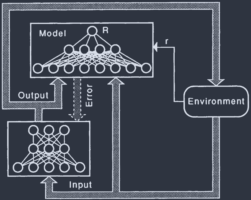
先训练 model, 再训练主网络, 使得 $R$ 最大.

通过 back-propagation 实现: 通过 $\delta = -R$ 传回主网络各单元独立的误差信号. 此时可使用常规的监督学习.

最小化 $(R-r)^{2}$ 的同时最大化 $r$. 最佳策略是优先训练 model network.

II:

average fluctuations from environment.
chase meaningless $r$ fluctuation
easy to maximize $R$.

III:

should exstimate a weighted average of the future reinforcement, for cumulative, not instantaneous value. (sacrifice shot-term reward for long-term gain)

critic: raw $r\overset{\text{critic}}{\to}$ processed signal $\rho$

reinforcement comparison: critic generate a prediction $R$ of $r$, could use $\rho = r-R$. ($\rho>0$: reward; $\rho<0$: penalty)

7.1 Boltzmann Machines(玻尔兹曼机)#

Stochastic Units(随机单元)#

Variations on Boltzmann Machines(玻尔兹曼机的变种)#

Statistical Mechanics Reformulation(统计力学重构)#

Deterministic Boltzmann Machines(确定性玻尔兹曼机)#

7.2 Recurrent Back-Propagation(递归反向传播)#

7.3 Learning Time Sequences(时间序列学习)#

Tapped Delay Lines(抽头延迟线)#

Context Units(上下文/记忆单元)#

Back-Propagation Through Time(时间反向传播)#

Real-Time Recurrent Learning(实时递归学习)#

Time-Dependent Recurrent Back-Propagation(含时递归反向传播)#

7.4 Reinforcement Learning(强化学习)#

Associative Reward-Penalty(联想奖惩) $A_{\text{RP}}$#

Theory of Associative Reward-Penalty(联想奖惩理论)#

Models & Critics#

7.1 Boltzmann Machines(玻尔兹曼机)

Stochastic Units(随机单元)

Variations on Boltzmann Machines(玻尔兹曼机的变种)

Statistical Mechanics Reformulation(统计力学重构)

Deterministic Boltzmann Machines(确定性玻尔兹曼机)

7.2 Recurrent Back-Propagation(递归反向传播)

7.3 Learning Time Sequences(时间序列学习)

Tapped Delay Lines(抽头延迟线)

Context Units(上下文/记忆单元)

Back-Propagation Through Time(时间反向传播)

Real-Time Recurrent Learning(实时递归学习)

Time-Dependent Recurrent Back-Propagation(含时递归反向传播)

7.4 Reinforcement Learning(强化学习)

Associative Reward-Penalty(联想奖惩) $A_{\text{RP}}$

Theory of Associative Reward-Penalty(联想奖惩理论)

Models & Critics