Abstract

The role of intrinsic cortical connections in processing sensory input and in generating behavioral output is poorly understood. We have examined this issue in the context of the tuning of neuronal responses in cortex to the orientation of a visual stimulus.

We analytically study a simple network model that incorporates both orientationselective input from the lateral geniculate nucleus and orientation-specific cortical interactions.

Depending on the model parameters, the network exhibits orientation selectivity that originates from within the cortex, by a symmetrybreaking mechanism. In this case, the width of the orientation tuning can be sharp even if the lateral geniculate nucleus inputs are only weakly anisotropic.

By using our model, several experimental consequences of this cortical mechanism of orientation tuning are derived. The tuning width is relatively independent of the contrast and angular anisotropy of the visual stimulus.

The transient population response to changing of the stimulus orientation exhibits a slow “virtual rotation.” Neuronal cross-correlations exhibit long time tails, the sign of which depends on the preferred orientations of the cells and the stimulus orientation.

皮层内在连接在处理感觉输入和生成行为输出中的作用尚不清楚. 我们在视觉刺激方向对皮层中神经元反应调制的背景下研究了这个问题.

我们分析性地研究了一个简单的网络模型, 该模型结合了来自外侧膝状体核的方向选择性输入和方向特异性皮层相互作用.

根据模型参数, 网络表现出源自皮层内部的方向选择性(通过一种 对称性破缺机制). 在这种情况下, 即使外侧膝状体核输入仅具有弱 各向异性, 方向调制的宽度也可以很窄.

通过使用我们的模型, 推导出了这种皮层方向调制机制的几个实验结果. 调制宽度相对独立于视觉刺激的对比度和角向各向异性.

对刺激方向变化的瞬态, 群体反应表现出缓慢的“虚拟旋转”. 神经元交叉相关表现出长时间尾, 其符号取决于细胞的 优选方向 和刺激方向.

Introduction

Neurons in the primary visual cortex respond preferentially to edges with a particular orientation. The input to the cortex is provided by neurons in the lateral geniculate nucleus (LGN), which respond independently of the stimulus orientation.

The mechanism for the generation of orientation selectivity in the cortex is not fully known.

初级视觉皮层中的神经元对具有特定方向的边缘有优先反应. 皮层的输入由 外侧膝状体核(LGN) 中的神经元提供, 这些神经元对刺激方向独立响应.

皮层中方向选择性产生的机制尚不完全清楚.

According to the classical model of Hubel and Wiesel, the preferred orientation (PO) of a cortical cell originates from the geometrical alignment of the circular receptive fields of the LGN neurons that are afferent to it.

The experimental evidence of this model is ambiguous. The alignment of the receptive fields of the LGN inputs to a cortical cell apparently parallels the cell’s PO .

However, suppression of cortical inhibition tends to considerably degrade orientation tuning, suggesting that cortical circuitry plays an important role in shaping the relatively sharp orientation tuning in the cortex.

根据 Hubel 和 Wiesel 的经典模型, 皮层细胞的 优选方向(PO) 源自传入该细胞的 LGN 神经元的圆形感受野的几何排列.

该模型的实验证据是模糊的. 传入皮层细胞的 LGN 输入的感受野排列显然与细胞的 PO 平行. 然而, 弱化 皮层抑制 倾向于显著降低 方向调制, 表明皮层回路在塑造皮层中相对尖锐的方向调制中起着重要作用.

Furthermore, estimates based on intracellular measurements indicate that most of the orientation-selective excitatory input to cortical cells comes from cortical feedback. Several models implicating cortical inhibition have been proposed (for reviews, see refs. 7 and 8).

此外, 基于细胞内测量的估计表明, 大多数对皮层细胞具有方向选择性的兴奋性输入来自 皮层反馈. 已经提出了几种涉及皮层抑制的模型(综述见参考文献7和8).

Their analysis, however, is hindered by the need to resort to massive numerical simulations of the different models. Computational complexity also precluded a detailed study of the role of the cortical excitatory connections.

An important constraint on modeling orientation selectivity, which has not yet been fully addressed, is the experimental finding that the tuning width is relatively insensitive to the contrast of the stimulus.

Most experimental and theoretical studies of orientation selectivity focus on the response properties of single neurons. However, valuable insight into the cooperativity among cortical neurons can be gained from measurements of the correlations between the responses of different neurons. Theoretical predictions regarding the magnitude and form of correlation functions in neuronal networks have been lacking.

然而, 它们的分析受到需要诉诸于不同模型的大规模数值模拟的阻碍. 计算复杂性也阻止了对皮层兴奋性连接作用的详细研究.

对建模方向选择性的一个重要限制是实验发现 调制宽度 对刺激对比度相对不敏感, 这一点尚未得到充分解决.

大多数关于方向选择性的实验和理论研究都集中在单个神经元的响应特性上. 然而, 通过测量不同神经元响应之间的相关性, 可以获得有关皮层神经元之间协作的重要见解. 关于神经网络中相关函数的大小和形式的理论预测一直缺乏.

Here we study mechanisms for orientation selectivity by using a simple neural network model that captures the gross architecture of primary visual cortex. By assuming simplified neuronal stochastic dynamics, the network properties have been solved analytically, thereby providing a useful framework for the study of the roles of the input and the intrinsic connections in the formation of orientation tuning in the cortex.

Furthermore, by using a recently developed theory of neuronal correlation functions in large stochastic networks, we have calculated the cross-correlations (CCs) between the neurons in the network.

We show that different models of orientation selectivity may give rise to qualitatively different spatiotemporal patterns of neuronal correlations. These predictions can be tested experimentally.

在这里, 我们使用一个简单的神经网络模型来研究方向选择性的机制, 该模型捕捉了初级视觉皮层的总体结构. 通过假设简化的神经元随机动力学, 网络属性已经被解析地解决, 从而为研究输入和内在连接在皮层中形成方向调制中的作用提供了有用的框架.

此外, 通过使用最近开发的大型随机网络中神经元相关函数的理论, 我们计算了网络中神经元之间的 交叉关联(CCs).

我们表明, 不同的方向选择性模型可能会产生定性上不同的神经元相关性的时空模式. 这些预测可以通过实验进行测试.

Model

We consider a network model with an architecture of a cortical hypercolumn.

It consists of $N_{E}$ excitatory neurons and $N_{I}$ inhibitory neurons that respond selectively to a small oriented visual stimulus in a common receptive field.

The neurons are parameterized by an angle $\theta$, ranging from $-\pi/2$ to $+\pi/2$, that denotes their POs.

The interaction between a presynaptic excitatory neuron $\theta^{\prime}$ and a postsynaptic excitatory or inhibitory neuron $\theta$ is equal to $N_{E}^{-1}E(\theta-\theta^{\prime})$.

Similarly, the interaction between a presynaptic inhibitory neuron and a postsynaptic neuron is $N_{I}^{-1}I(\theta-\theta^{\prime})$.

The functions $E(\theta-\theta^{\prime})$ and $I(\theta-\theta^{\prime})$ represent the fact that the strength of the interactions between two orientation columns depends on the difference between their POs.

The synaptic input from the LGN to a neuron $\theta$ is denoted as $h^{\text{ext}}(\theta-\theta_{0})$, where $\theta_{0}$ is the orientation of the external stimulus.

我们考虑一个具有皮层超柱结构的网络模型.

它由 $N_{E}$ 个 兴奋性神经元 和 $N_{I}$ 个 抑制性神经元 组成, 这些神经元选择性地响应 共同感受野 中的小定向视觉刺激.

神经元由一个角度 $\theta$ 参数化, 范围从 $-\pi/2$ 到 $+\pi/2$, 表示它们的 PO.

一个突触前兴奋性神经元 $\theta^{\prime}$ 和一个突触后兴奋性或抑制性神经元 $\theta$ 之间的相互作用等于 $N_{E}^{-1}E(\theta-\theta^{\prime})$.

类似地, 一个突触前抑制性神经元和一个突触后神经元之间的相互作用是 $N_{I}^{-1}I(\theta-\theta^{\prime})$.

函数 $E(\theta-\theta^{\prime})$ 和 $I(\theta-\theta^{\prime})$ 表示两个方向柱之间相互作用的强度, 具体取决于它们 PO 之间的差异.

从 LGN 到神经元 $\theta$ 的 突触输入 表示为 $h^{\text{ext}}(\theta-\theta_{0})$, 其中 $\theta_{0}$ 是外部刺激的方向.

Neurons switch stochastically between a quiescent state [denoted as $S(\theta) = 0$], representing a state with background firing rate ($\approx 5$ spikes per sec), and an active state [$S(\theta) = 1$], representing a state with saturated firing rate (~500 spikes per sec).

神经元在静息状态[表示为 $S(\theta) = 0$]和激活状态[$S(\theta) = 1$]之间随机切换, 分别表示具有背景发射率(约每秒 5 个峰值)和饱和发射率(约每秒 500 个峰值)的状态.

The transition rates between these states are governed by a sigmoidal gain function, $g[h(\theta, t)]$, where $h(\theta, t)$ is the total synaptic input to the neuron $\theta$ at time $t$.

这些状态之间的转换速率由 sigmoid 增益函数 $g[h(\theta, t)]$ 控制, 其中 $h(\theta, t)$ 是 $t$ 神经元 $\theta$ 的总突触输入.

By assuming that the number of neurons is large and that they cover uniformly all the angles, the activity profile in the network at time $t$ can be represented by a continuous function $m(\theta,t)$, $0\leq m\leq 1$.

This function denotes the mean activity level, relative to the saturation activity level, of the neurons with POs in the neighborhood of $\theta$, at time $t$.

Note that since the synaptic inputs to the excitatory and the inhibitory neurons in our model are the same, $m(\theta, t)$ describes the mean activity levels of both types of neurons.

通过假设神经元数量充分大而均匀覆盖所有角度, 网络中 $t$ 时刻的活动曲线形状可以表示为连续函数 $m(\theta,t)$, 其中 $0\leq m\leq 1$.

该函数表示在时间 $t$ 时, PO 在 $\theta$ 附近的神经元的平均活动水平, 相对于饱和活动水平.

请注意, 由于我们模型中兴奋性和抑制性神经元的突触输入相同, $m(\theta, t)$ 描述了两种类型神经元的平均活动水平.

In the limit of a large network, $m(\theta,t)$ obeys the following deterministic mean-field equations:

$$ \tau_{0}\frac{\mathrm{d}}{\mathrm{d}t}m(\theta, t) = -m(\theta, t) + g[h(\theta, t)] $$

where $\tau_{0}$ is a microscopic characteristic time(a few milliseconds), and the total synaptic input $h(\theta, t)$ is

$$ h(\theta, t) = \int^{+\pi/2}_{-\pi/2}\frac{\mathrm{d}\theta^{\prime}}{\pi}J(\theta-\theta^{\prime})m(\theta^{\prime},t) + h^{\text{ext}}(\theta-\theta_{0}) $$

Here $J(\theta-\theta^{\prime})$ represents the net interaction between neurons $\theta$ and $\theta^{\prime}$, ie., $J(\theta-\theta^{\prime}) = E(\theta-\theta^{\prime}) + I(\theta-\theta^{\prime})$.

在取大网络的极限下, $m(\theta,t)$ 遵循以下确定性平均场方程:

$$ \tau_{0}\frac{\mathrm{d}}{\mathrm{d}t}m(\theta, t) = -m(\theta, t) + g[h(\theta, t)] $$

其中 $\tau_{0}$ 是一个微观特征时间(几毫秒), 总突触输入 $h(\theta, t)$ 为

$$ h(\theta, t) = \int^{+\pi/2}_{-\pi/2}\frac{\mathrm{d}\theta^{\prime}}{\pi}J(\theta-\theta^{\prime})m(\theta^{\prime},t) + h^{\text{ext}}(\theta-\theta_{0}) $$

这里 $J(\theta-\theta^{\prime})$ 表示神经元 $\theta$ 和 $\theta^{\prime}$ 之间的净相互作用, 即 $J(\theta-\theta^{\prime}) = E(\theta-\theta^{\prime}) + I(\theta-\theta^{\prime})$.

We choose $E(\theta) = E_{0} + E_{2}\cos{(2\theta)}$ and $I(\theta) = -I_{0}-I_{2}\cos{(2\theta)}$ with $E_{0}\geq E_{2}\geq 0$, $I_{0}\geq I_{2}\geq 0$. This choice implies that both the excitatory interactions and the inhibitory interactions are maximal for orientation columns with similar POs. This is in accord with the observation that the excitatory and inhibitory postsynaptic potentials to a cell have similar tuning. The net interaction is

$$ J(\theta) = -J_{0} + J_{2}\cos{(2\theta)} $$

with $J_{0} = I_{0} - E_{0}$ and $J_{2} = E_{2} - I_{2}$, both assumed to be positive. The constant $J_{0}$ represents a uniform all-to-all inhibition; $J_{2}$ measures the amplitude of the orientation-specific part of the interaction.

Neurons with similar POs are more strongly coupled excitatorily than neurons with dissimilar ones.

我们选择 $E(\theta) = E_{0} + E_{2}\cos{(2\theta)}$ 和 $I(\theta) = -I_{0}-I_{2}\cos{(2\theta)}$, 其中 $E_{0}\geq E_{2}\geq 0$, $I_{0}\geq I_{2}\geq 0$. 这种选择意味着对于具有相似 PO 的方向柱, 兴奋性相互作用和抑制性相互作用都是最大的. 这与对细胞的兴奋性和抑制性突触后电位具有类似调制的观察结果是一致的. 净相互作用为

$$ J(\theta) = -J_{0} + J_{2}\cos{(2\theta)} $$

其中 $J_{0} = I_{0} - E_{0}$ 和 $J_{2} = E_{2} - I_{2}$, 两者均假定为正. 常数 $J_{0}$ 表示均匀的 全连接抑制; $J_{2}$ 测量了相互作用的方向特异性部分的幅度.

具有相似 PO 的神经元之间的兴奋性耦合比具有不同 PO 的神经元更强.

The external input is taken as

$$ h^{\text{ext}}(\theta) = c[1-\epsilon+\epsilon\cos{(2\theta)}] $$

with $0\leq \epsilon \leq 1/2$. The parameter $\epsilon$ denotes the magnitude of the angular anisotropy of the input. The case $\epsilon=0$ denotes the limit where the input to the cortex is fully isotropic. The coefficient $c$ measures the average amplitude of the input and will be referred to as the stimulus contrast.

Finally, we use a semilinear gain function, i.e., $g(h) = 0$ for $h\leq T$, $g(h) = \beta(h - T)$ for $h\geq T$, and $g(h) = 1$ for $h\geq T+\beta^{-1}$. The parameter $T$ is the threshold, which will be taken as 1, and $\beta$ is the gain factor.

外部输入取为

$$ h^{\text{ext}}(\theta) = c[1-\epsilon+\epsilon\cos{(2\theta)}] $$

其中 $0\leq \epsilon \leq 1/2$. 参数 $\epsilon$ 表示输入的角向各向异性的大小. $\epsilon=0$ 的情况表示皮层输入完全各向同性的极限. 系数 $c$ 测量输入的平均幅度, 将被称为刺激对比度.

最后, 我们使用半线性增益函数, 即对于 $h\leq T$, $g(h) = 0$, 对于 $h\geq T$, $g(h) = \beta(h - T)$, 对于 $h\geq T+\beta^{-1}$, $g(h) = 1$. 参数 $T$ 是阈值, 将取为 1, $\beta$ 是增益因子.

This reflects the experimental finding that neuronal responses exhibit a sharp threshold contrast below which they vanish. Above threshold the mean firing rate of the neuron increases roughly linearly with the contrast. The slope of this rise is represented in our model by the constant $\beta$.

Finally, the response saturates at high contrasts. The particular functional forms of the interactions, the LGN input and the gain function were chosen for the sake of simplicity. More general forms yield a behavior that is qualitatively similar to the present model.

这反映了实验发现神经元响应表现出一个尖锐的阈值对比度, 低于该对比度响应消失. 在阈值以上, 神经元的平均发射率大致与对比度线性增加. 我们模型中这种上升的斜率由常数 $\beta$ 表示.

最后, 响应在高对比度下 饱和. 为了简化起见, 相互作用、LGN 输入和增益函数都选取了特定函数形式. 对于更一般的形式, 则在定性上与目前模型类似.

Mechanisms for Orientation Selectivity

Mean-Field Solution

In the steady state, $m(\theta)$ is of the form $m(\theta) = M(\theta - \theta_{0})$, where $M(\theta)$ peaks at $\theta = 0$. It represents the activity profile of the network relative to the orientation of the stimulus. Thus, $M(\theta)$ also represents the tuning curve of a neuron, centered at its PO.

在稳态下, $m(\theta)$ 的形式为 $m(\theta) = M(\theta - \theta_{0})$, 其中 $M(\theta)$ 在 $\theta = 0$ 处达到峰值. 它表示相对于刺激方向的网络活动曲线. 因此, $M(\theta)$ 也表示以其 PO 为中心的神经元的调制曲线.

This function is given by the solution of the mean-field equation $M(\theta) = g[H(\theta)]$ with $H(\theta)$ being the local field, Eq. 2, centered at $\theta_{0}$. Its value is $H(\theta) = (\epsilon c + J_{2}m_{2})\cos{(2\theta)} + c(1 - \epsilon) - J_{0}m_{0}$, where $m_{0}$ and $m_{2}$ are the zeroth and the second Fourier coefficients of $M(\theta)$.

该函数由平均场方程 $M(\theta) = g[H(\theta)]$ 的解给出, 其中 $H(\theta)$ 是以 $\theta_{0}$ 为中心的局部场, 见方程2. 其值为 $H(\theta) = (\epsilon c + J_{2}m_{2})\cos{(2\theta)} + c(1 - \epsilon) - J_{0}m_{0}$, 其中 $m_{0}$ 和 $m_{2}$ 分别是 $M(\theta)$ 的零阶和二阶傅里叶系数.

The order parameter $m_{0}$ measures the neuronal activity averaged over the whole network, whereas $m_{2}$ measures the variation of this activity across the different columns.

Self-consistent equations for $m_{0}$ and $m_{2}$ are derived by evaluating the Fourier transform of $M(\theta)$. The resultant form of $M(\theta)$ is $M(\theta) = \beta(\epsilon c + J_{2}m_{2})[\cos{(2\theta)} - \cos{(2\theta_{c})}]$ for $|\theta| < \theta_{C}$ and zero otherwise (see examples in Fig. 2). The cutoff angle $\theta_{C}$, which is determined by the condition $H(\pm\theta_{C}) = 1$, is half of the full width of the tuning curve and will be denoted as the tuning width.

The above solution holds for suprathreshold contrast, $c > 1$. Otherwise, $M(\theta)$ is zero. In the following, we study the orientation tuning properties of the steady-state solution. In particular, we examine the dependence of the tuning width on the stimulus contrast, $c$, and anisotropy, $\epsilon$, for different ranges of values of the connectivity parameters.

序参量 $m_{0}$ 测量整个网络中神经元活动的平均值, 而 $m_{2}$ 测量不同柱之间这种活动的变化.

通过计算 $M(\theta)$ 的傅里叶变换, 得到了 $m_{0}$ 和 $m_{2}$ 的自洽方程. $M(\theta)$ 的结果形式为 $M(\theta) = \beta(\epsilon c + J_{2}m_{2})[\cos{(2\theta)} - \cos{(2\theta_{c})}]$ 对于 $|\theta| < \theta_{C}$, 否则为零(见图 2 中的示例). 截止角 $\theta_{C}$ 由条件 $H(\pm\theta_{C}) = 1$ 决定, 是调制曲线全宽度的一半, 被称为调制宽度.

上述解适用于超阈值对比度, 即 $c > 1$. 否则, $M(\theta)$ 为零. 在下文中, 我们研究稳态解的方向调制特性. 特别地, 我们检查在不同连接参数值范围内, 调制宽度对刺激对比度 $c$ 和各向异性 $\epsilon$ 的依赖性.

Hubel and Wiesel Scenario

The simplest scenario for orientation tuning is based on the Hubel-Wiesel mechanism. In the context of our model, this scenario corresponds to the case where the only synaptic input is coming from the LGN and this input is strongly anisotropic.

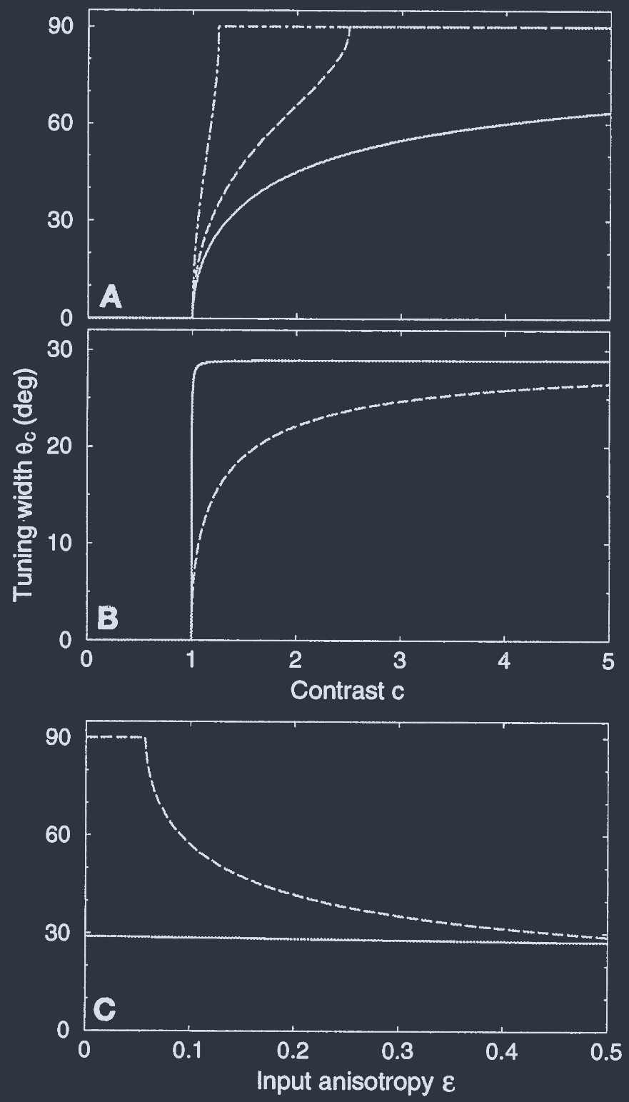
Hence, the cortical local interaction $J(\theta)$ is zero and $\epsilon$ is substantially bigger than zero. The dependence of the tuning width $\theta_{C}$ on $c$ in this case is shown in Fig. 1A for different values of $\epsilon$. Near threshold (i.e., for $c\to 1$), $\theta_{C}$ vanishes, signaling the sharpening of the tuning width, relative to the input, by the thresholding operation of the cortical neurons.

This, however, results in a strong dependence of the width on the contrast. As $c$ increases, $\theta_{C}$ grows and beyond a certain value saturates at its maximum value $\pi/2$, which corresponds to the situation where all the neurons are activated by all stimuli.

方向调制的最简单情景基于 Hubel-Wiesel 机制. 在我们模型的背景下, 这种情景对应于唯一的突触输入来自 LGN 并且该输入具有强各向异性.

因此, 皮层局部相互作用 $J(\theta)$ 为零, 并且 $\epsilon$ 显著大于零. 图 1A 显示了在这种情况下, 不同 $\epsilon$ 值下调制宽度 $\theta_{C}$ 对 $c$ 的依赖性. 在阈值附近(即对于 $c\to 1$), $\theta_{C}$ 消失, 表明通过皮层神经元的阈值操作, 相对于输入, 调制宽度变窄.

然而, 这导致宽度对对比度的强依赖性. 随着 $c$ 的增加, $\theta_{C}$ 增长, 并且超过某个值后饱和在其最大值 $\pi/2$, 这对应于所有神经元都被所有刺激激活的情况.

Uniform Inhibition

A simple cortical mechanism for sharpening the orientation tuning is based on isotropic cortical inhibition.

This scenario corresponds in our model to $J_{0} > 0$ and $J_{2} = 0$. In this case, the external input of each neuron has to overcome an effective enhanced threshold that increases with $c$ because of the increase of the inhibitory feedback.

基于 各向同性皮层抑制 的方向调制锐化的简单皮层机制.

在我们的模型中, 这种情景对应于 $J_{0} > 0$ 和 $J_{2} = 0$. 在这种情况下, 由于抑制反馈的增加, 每个神经元的外部输入必须克服一个随 $c$ 增加的有效增强阈值.

Thus, even for $c\gg 1$, the inhibition may provide a sufficiently potent threshold to sharpen the tuning width. This is clearly seen in Fig. 1B (dashed line).

Nevertheless, there is a strong dependence of the width on the contrast $c$. In addition, the width depends strongly on the anisotropy of the input, $\epsilon$. In particular, when $\epsilon$ is small, $\theta_{C} = \pi/2$ for large $c$. This is shown in Fig. 1C (dashed line).

因此, 即使对于 $c\gg 1$, 抑制也可能提供足够强大的阈值来锐化调制宽度. 这在图1B(虚线)中清晰可见.

然而, 宽度强烈依赖于对比度 $c$. 此外, 宽度还强烈依赖于输入的 各向异性 $\epsilon$. 特别是, 当 $\epsilon$ 很小时, 对于大 $c$, $\theta_{C} = \pi/2$. 这在图 1C(虚线)中显示.

Marginal Phase

In the cases studied above, the anisotropy of the input to the cortex is the only source of orientation specificity. Can orientation specificity be generated by cortical interactions alone-even in the absence of significant anisotropy in the external input?

在上述研究的情况下, 皮层输入的各向异性是方向特异性的唯一来源. 即使在外部输入没有显著各向异性的情况下, 方向特异性也能仅由皮层相互作用产生吗？

To answer this question, we have studied the case of $\epsilon = 0$ with $J_{0}$ and $J_{2} > 0$.

The assumed rotational symmetry of the cortex implies that when $\epsilon = 0$, there is always a homogeneous solution, $M(\theta) = m_{0}$, which agrees with the naive expectation that the orientation tuning disappears when the external stimulus is isotropic.

However, the equations yield also an inhomogeneous solution, provided that the angular modulation of the cortical interactions, $J_{2}$, is big enough, $J_{2} > 2/\beta$. This solution represents a spontaneous generation of orientation tuning. It can be written as $m(\theta) = M(\theta - \phi)$, where the angle $\phi$, which determines the location of the peak in $m(\theta)$, is arbitrary.

为了回答这个问题, 我们研究了 $\epsilon = 0$ 且 $J_{0}$ 和 $J_{2} > 0$ 的情况.

假设的皮层旋转对称性意味着当 $\epsilon = 0$ 时, 总是存在一个均匀解 $M(\theta) = m_{0}$, 这与外部刺激各向同性时方向调制消失的朴素预期是一致的.

然而, 只要皮层相互作用的角向调制 $J_{2}$ 足够大, 即 $J_{2} > 2/\beta$, 方程还会产生一个非均匀解. 该解表示方向调制的自发生成. 它可以写成 $m(\theta) = M(\theta - \phi)$, 其中角度 $\phi$ 决定了 $m(\theta)$ 峰值的位置, 是任意的.

This means that there is a continuum of stable states: they all have identical orientation tuned activity profiles, but they differ in the location of their peaks. The overall magnitude of $m(\theta)$ is determined by $c$ but the shape of the activity profile is determined only by the cortical interactions.

In particular, the width of $m(\theta)$ is independent of $c$ but strongly depends on the magnitude of $J_{2}$. The bigger $J_{2}$, the smaller the width. We denote this solution a marginal phase because there are no barriers between the different attractors.

This implies that the motion from one attractor to another is easier than motions in other directions of phase space. When the marginal solution exists, the naive homogeneous solution is unstable.

这意味着存在一系列连续的稳定状态: 它们都有相同的方向调制活动曲线形状, 只是峰值位置不同. $m(\theta)$ 的整体幅度由 $c$ 决定, 但活动曲线的形状仅由皮层相互作用决定.

特别是, $m(\theta)$ 的宽度独立于 $c$, 但强烈依赖于 $J_{2}$ 的大小. $J_{2}$ 越大, 宽度越小. 我们将这种解称为 边际相, 因为不同吸引子之间没有障碍.

这意味着从一个吸引子到另一个吸引子的运动比在相空间的其他方向上的运动更容易. 当边际解存在时, 朴素的均匀解是不稳定的.

In reality, the location of the peak of the activity is not arbitrary but is determined by the orientation of the external input.

Therefore, in a realistic implementation of the last scenario $\epsilon$ should be assumed to be small but nonzero.

Since $\epsilon$ is small, the main effect of the anisotropy of the input is to select among the continuum of possible states that state in which the location of the peak in the activity matches theorientation of the stimulus, but it will not affect the shape of the tuning curve very much. This is indeed borne out by a solution of the mean-field equations with a small nonzero $\epsilon$ and large $J_{0}$ and $J_{2}$.

在现实中, 活动峰值的位置不是任意的, 而是由外部输入的方向决定的.

因此, 在最后一种情景的现实实现中, $\epsilon$ 应假设为小量但非零.

由于 $\epsilon$ 很小, 输入各向异性的主要作用是在可能状态的连续体中选择一个状态, 即活动峰值的位置与刺激方向匹配, 但它不会太影响调制曲线的形状. 通过对具有小非零 $\epsilon$ 和大 $J_{0}$ 及 $J_{2}$ 的平均场方程求解, 确实验证了这一点.

There is a unique stable state, $m(\theta) = M(\theta - \theta_{0})$, where $M(\theta)$ is approximately the same as for $\epsilon = 0$.

Whereas when $\epsilon = 0$, $\theta_{C}$ was independent of $c$, and when $\epsilon$ is nonzero, $\theta_{C}$ vanishes as $c\to 1$. However, this decrease in $\theta_{C}$ occurs in a very narrow range of $c$ near threshold, $c - 1 = O(\epsilon)$, as shown in Fig. 1B (solid line).

The value of $\theta_{C}$ for larger $c$ is independent of $c$. It is also insensitive to changes in the value of $\epsilon$, as shown in Fig. 1C (solid line).

存在一个唯一稳定状态 $m(\theta) = M(\theta - \theta_{0})$, 其中 $M(\theta)$ 大致与 $\epsilon = 0$ 时相同.

当 $\epsilon = 0$ 时, $\theta_{C}$ 独立于 $c$, 而当 $\epsilon$ 非零时, $\theta_{C}$ 在 $c\to 1$ 时消失. 然而, 如图 1B (实线)所示, 这种 $\theta_{C}$ 的减小发生在阈值附近的非常狭窄的 $c$ 范围内, 即 $c - 1 = O(\epsilon)$.

较大 $c$ 时的 $\theta_{C}$ 值独立于 $c$. 如图 1C (实线)所示, 它对 $\epsilon$ 值的变化也不敏感.

Fic. 1. Dependence of the orientation tuning with $\theta_{C}$ on the stimulus contrast and input anisotropy, for different mechanisms of tuning. The angle $\theta_{C}$ is the half-width of the tuning curve: neurons with POs of $>\theta_{C}$ away from the stimulus orientation are not activated.

(A) The Hubel-Wiesel model, where the cortical interaction parameters $J_{0}$ and $J_{2}$ are zero. The tuning width is plotted against the contrast of the visual stimulus, $c$, for different values of the input anisotropy param- eter, $\epsilon:\epsilon = 0.1, 0.3$, and $0.5$ (dot-dashed, dashed, and solid lines, respectively). For $\epsilon < 0.5$, there is a critical value of $c$ above which $\theta_{C} = \pi/2$, meaning that all neurons are activated by all stimuli. In the range where $\theta_{C}$ is small, it strongly depends on the level of contrast. Note that $\epsilon = 0.5$ is the maximal value of anisotropy in our model. Here and in Figs. 2 and 3, $\beta = 0.1$.

(B) Effect of cortical interactions on the tuning width. Dashed curve is for uniform cortical inhibition, with $\epsilon = 0.5$, $J_{0} = 155$, and $J_{2} = 0$. The solid line is for parameters close to the marginal phase, where the tuning is dominated by the cortical interactions. In this case, $\theta_{C}$ saturates quickly to $\approx 30°$, while the level of maximal activity is still far from saturation (data not shown). Parameters are $\epsilon = 0.01$, $J_{0} = 86$, and $J_{2} = 112$. They were chosen so that the value of $\theta_{C}$ agrees with the average value of the half-width for simple cells in the cat visual cortex.

(C) The tuning width as a function of the input anisotropy in the limit $c\gg 1$. The solid line is for the marginal phase; the dashed curve is for the Hubel-Wiesel mechanism with uniform cortical inhibition. Parameters are as in B.

图 1. 不同调制机制下, 调制宽度 $\theta_{C}$ 对刺激对比度和输入各向异性的依赖性. 角度 $\theta_{C}$ 是调制曲线的半宽度: PO 与刺激方向相差 $>\theta_{C}$ 的神经元不会被激活.

(A) Hubel-Wiesel 模型, 其中皮层相互作用参数 $J_{0}$ 和 $J_{2}$ 为零. 调制宽度与视觉刺激对比度 $c$ 的关系绘制在不同输入各向异性参数 $\epsilon$ 下: $\epsilon = 0.1, 0.3$ 和 $0.5$（分别为点划线、虚线和实线）. 对于 $\epsilon < 0.5$, 存在一个临界值的 $c$, 超过该值时 $\theta_{C} = \pi/2$, 意味着所有神经元都被所有刺激激活. 在 $\theta_{C}$ 较小的范围内, 它强烈依赖于对比度水平. 请注意, $\epsilon = 0.5$ 是我们模型中各向异性的最大值. 在此图和图 2 及图 3 中, $\beta = 0.1$.

(B) 皮层相互作用对调制宽度的影响. 虚线 曲线表示均匀皮层抑制, 参数为 $\epsilon = 0.5$, $J_{0} = 155$ 和 $J_{2} = 0$. 实线 表示接近边际相的参数, 其中调制由皮层相互作用主导. 在这种情况下, $\theta_{C}$ 快速饱和至约 30°, 而最大活动水平仍远未饱和(数据未显示). 参数为 $\epsilon = 0.01$, $J_{0} = 86$ 和 $J_{2} = 112$. 它们被选择使得 $\theta_{C}$ 的值与猫视觉皮层中简单细胞的半宽度平均值一致.

(C) 在 $c\gg 1$ 极限下, 调制宽度作为输入各向异性的函数. 实线表示边际相; 虚线曲线表示具有均匀皮层抑制的 Hubel-Wiesel 机制. 参数如 B 所示.

Virtual Rotation

An interesting difference between the scenarios described above appears in the time-dependent response of the system to a change in the orientation of the external stimulus.

Consider the case where the orientation of the external stimulus is changed at time 0 from $\theta_{0}=\theta_{1}$ to $\theta_{0} = \theta_{2}$.

We assume that initially the stimulus was present long enough so that the system reached a steady-state $m(\theta)$ with a peak at $\theta = \theta_{1}$.

在上述情景之间, 一个有趣的区别出现在系统对外部刺激方向变化的含时响应中.

考虑在时刻 0 时外部刺激的方向从 $\theta_{0}=\theta_{1}$ 变为 $\theta_{0} = \theta_{2}$ 的情况.

我们假设最初刺激存在的时间足够长, 以使系统达到峰值在 $\theta = \theta_{1}$ 处的稳态 $m(\theta)$.

How will the population activity respond to the change in orientation?

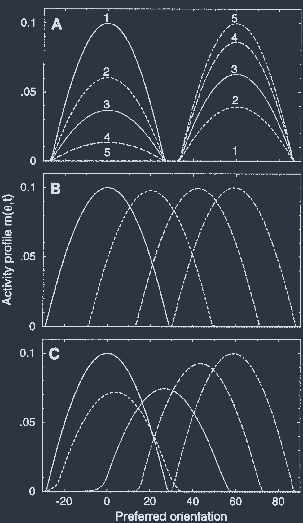
In the case of isotropic cortical interactions ($J_{2} = 0$), the initial activity profile that peaked at $\theta_{1}$, decays in magnitude while another profile peaked at $\theta_{2}$ grows, as shown in Fig. 2A.

In the marginal phase, the response is drastically different. The population activity is $m(\theta, t)\approx M[\theta - \phi(t)]$, where $M(\theta)$ is the activity profile at steady state. We denote this solution as virtual rotation.

群体活动将如何响应方向的变化？

在 各向同性皮层相互作用 ($J_{2} = 0$) 的情况下, 最初在 $\theta_{1}$ 处达到峰值的活动轮廓, 其幅度衰减, 而另一个在 $\theta_{2}$ 取峰值的曲线增长, 如图 2A 所示.

在 边际相 中, 响应截然不同. 群体活动为 $m(\theta, t)\approx M[\theta - \phi(t)]$, 其中 $M(\theta)$ 是稳态下的活动曲线. 我们将这种解称为虚拟旋转.

The activity at time $t$ is similar to that that would occur if there was an external stimulus with an orientation $\theta_{0} = \phi(t)$.

Substituting this form for $m(\theta, t)$ in the dynamic equations (Eqs. 1 and 2), we find that the variable $\phi(t)$ obeys $\dot{\phi}(t) \approx - \omega_{0}\sin{[2\phi(t) - 2\theta_{2}]}$, with $\phi(t = 0) = \theta_{1}$. The angular frequency $\omega_{0}$ is given by

$$ \omega_{0}\tau_{0} = \epsilon c/(2J_{2}m_{2}) $$

where $m_{2}$ is the second Fourier coefficient of $M(\theta)$.

$t$ 时刻的活动, 类似于外部刺激的方向为 $\theta_{0} = \phi(t)$ 的情况.

将这种形式的 $m(\theta, t)$ 代入动态方程(方程 1 和 2), 我们发现变量 $\phi(t)$ 遵循 $\dot{\phi}(t) \approx - \omega_{0}\sin{[2\phi(t) - 2\theta_{2}]}$, 其中 $\phi(t = 0) = \theta_{1}$. 角频率 $\omega_{0}$ 由下式给出

$$ \omega_{0}\tau_{0} = \epsilon c/(2J_{2}m_{2}) $$

其中 $m_{2}$ 是 $M(\theta)$ 的二阶傅里叶系数.

Note that in the marginal phase $m_{2}$ remains finite even for small $\epsilon$.

Thus, $\omega_{0}$, the angular velocity of the activity profile, is determined by the ratio of the modulation amplitudes of the external input and of the cortical synaptic input.

This result is valid provided $\omega_{0}\tau_{0} = O(\epsilon)\ll 1$. An example is shown in Fig. 2B, which corresponds to a marginal phase with $\epsilon = 0.01$. The activity profile moves with an (initial) angular velocity $0.2°/\tau_{0}$, without significant change in its shape.

Fig. 2C shows the case of $\epsilon = 0.1$. Here, the angular velocity is faster by an order of magnitude, as predicted by Eq. 5. In this case, the propagation of the activity is accompanied by significant transient changes in the amplitude of the activity profile.

请注意, 在边际相中, 即使对于小 $\epsilon$, $m_{2}$ 仍然是有限的.

因此, 活动曲线的角速度 $\omega_{0}$ 由外部输入和皮层突触输入的调制幅度之比决定.

该结果在 $\omega_{0}\tau_{0} = O(\epsilon)\ll 1$ 时有效. 图 2B 显示了一个例子, 对应于 $\epsilon = 0.01$ 的 边际相. 活动曲线以初始角速度 $0.2°/\tau_{0}$ 移动, 而其形状没有显著变化.

图 2C 显示了 $\epsilon = 0.1$ 的情况. 在这种情况下, 角速度比方程 5 预测的快一个数量级. 在这种情况下, 活动的传播伴随着活动曲线幅度的显著瞬态变化.

Fıc.2. Evolution ofneuronal activity in response to a change in the stimulus orientation from an initial value $\theta_{1} = 0°$ to $\theta_{2} = 60°$. The change occurs at $t = 0$.

(A) Hubel-Wiesel model with uniform inhibition. The activity profile centered at $0°$ decays while a new one, centered around $60°$, grows. Neurons in intermediate columns (e.g., with $0 = 30°$) stay in the quiescent state during the whole process. The time constant of the decay and growth is $\tau_{0}$. Times are 0, 0.5, 1, 2, and 6 $\tau_{0}$ (lines 1-5, respectively). Parameters are as in Fig. 1B (dashed line) and $c = 5$. For this value of contrast, the maximal activity level relative to saturation is 0.1, which corresponds to a rate of $\approx 50$ spikes per sec.

(B) Virtual rotation in the marginal phase. The activity profile moves toward $\theta_{2}$, activating successively the intermediate columns, and undergoing only very small changes during the process. $c = 1.678$; other parameters are as in Fig. 1B (solid line). Times are (left to right) 0, 90, 210, and 600 $\tau_{0}$.

(C) Virtual rotation accompanied by deformations in the activity profile. The magnitude of the deformations depends on the magnitude of $\epsilon$. Here $\epsilon = 0.1$, $J_{0} = 73$, $J_{2} = 110$, and $c = 1.45$. Times are (left to right) 0, 2, 10, 20, and 60 $\tau_{0}$. By assuming $\tau_{0} = 5\text{ msec}$, the predicted rotation velocity is 200 to 400°/sec.

图2. 神经元活动对刺激方向从初始值 $\theta_{1} = 0°$ 变为 $\theta_{2} = 60°$ 的响应演化. 变化发生在 $t = 0$.

(A) 具有均匀抑制的 Hubel-Wiesel 模型. 以 $0°$ 为中心的活动轮廓衰减, 而以 $60°$ 为中心的新轮廓增长. 在整个过程中, 中间柱(例如, $0 = 30°$)的神经元保持静止状态. 衰减和增长的时间常数为 $\tau_{0}$. 时间分别为 0、0.5、1、2 和 6 $\tau_{0}$（分别为线1-5）. 参数如图1B(虚线)所示, 且 $c = 5$. 对于该对比度值, 相对于饱和的最大活动水平为0.1, 对应于约每秒50次尖峰率.

(B) 边际相中的虚拟旋转. 活动轮廓向 $\theta_{2}$ 移动, 依次激活中间柱, 并在过程中仅经历非常小的变化. $c = 1.678$; 其他参数如图 1B (实线)所示. 时间分别为（从左到右）0、90、210 和 600 $\tau_{0}$.

(C) 活动轮廓伴随变形的虚拟旋转. 变形幅度取决于 $\epsilon$ 的大小. 这里 $\epsilon = 0.1$, $J_{0} = 73$, $J_{2} = 110$, 且 $c = 1.45$. 时间分别为（从左到右）0、2、10、20 和 60 $\tau_{0}$. 假设 $\tau_{0} = 5\text{ msec}$, 预测的旋转速度为 200 至 400°/秒.

CCs

The CC function $C(\theta,\theta^{\prime};\tau)$ measures the correlation between the temporal fluctuations in the rate of activity of a neuron $\theta$ at time $t$ and that of another neuron, $\theta^{\prime}$, at $t + \tau$. In our model, these fluctuations arise from the underlying stochasticity of the neuronal dynamics.

CC 函数 $C(\theta,\theta^{\prime};\tau)$ 测量时间 $t$ 时神经元 $\theta$ 的活动率涨落与另一神经元 $\theta^{\prime}$ 在 $t + \tau$ 时的活动率涨落之间的相关性. 在我们的模型中, 这些涨落源自神经元动力学的潜在随机性.

The deterministic mean-field equations, Eq. 1, neglect these small fluctuations.

To study the CCs induced by these fluctuations, we have applied a recently developed theory of correlations in stochastic neural networks and calculated analytically the CCs in our model for various parameter regimes.

确定性的平均场方程, 见方程 1, 忽略了这些小涨落.

为了研究这些涨落引起的 CCs, 我们应用了最近开发的 随机神经网络相关性理论, 并在各种参数范围内分析计算了我们模型中的 CCs.

We consider here the CCs between excitatory neurons in the case of uniform inhibition and in the marginal phase.

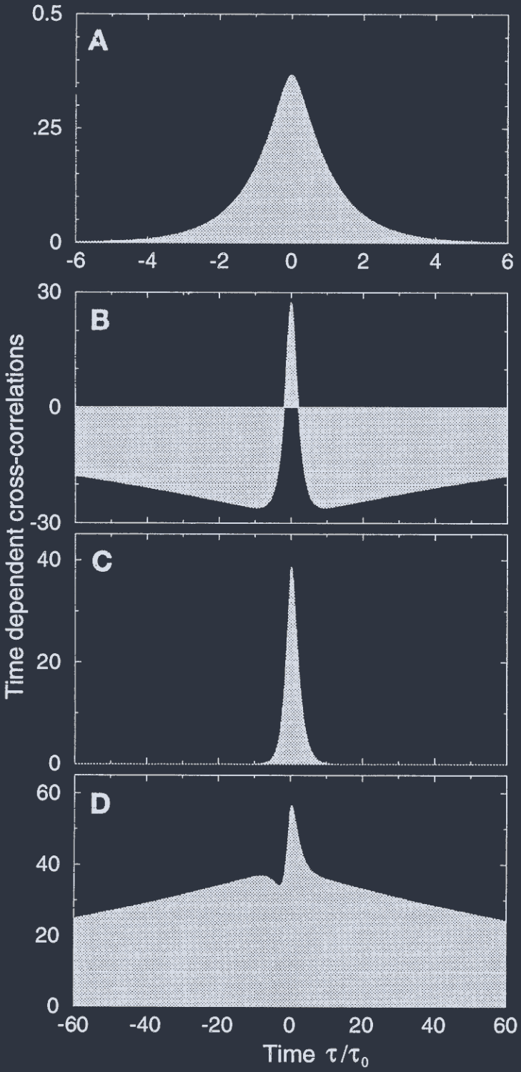
In the uniform inhibition case, the CCs are independent of $\theta$, $\theta^{\prime}$, and $\theta_{0}$, as long as the two neurons are activated by the stimulus, and the CCs decay on a fast time scale, of the order of the microscopic time constant $\tau_{0}$. This is shown in Fig. 3A.

The results for the marginal phase are drastically different. Here, in addition to fast-decaying components, the CCs possess also a slow component that has the following unique dependence on $\theta$, $\theta^{\prime}$, and $\theta_{0}$,

$$ C(\theta,\theta^{\prime};\tau) \propto \frac{1}{\epsilon}\sin{(2\theta-2\theta_{0})}\sin{(2\theta^{\prime}-2\theta_{0})}\exp{(-\epsilon|\tau|/\tau_{0})} $$

我们在这里考虑均匀抑制和边际相情况下兴奋性神经元之间的 CCs.

在均匀抑制情况下, 只要两个神经元被刺激激活, CCs 独立于 $\theta$、$\theta^{\prime}$ 和 $\theta_{0}$, 并且 CCs 在快速时间尺度上衰减, 其数量级为微观时间常数 $\tau_{0}$. 如图 3A 所示.

边际相的结果截然不同. 在这里, 除了快速衰减的分量外, CCs 还具有一个缓慢分量, 其对 $\theta$、$\theta^{\prime}$ 和 $\theta_{0}$ 具有以下独特依赖性,

$$ C(\theta,\theta^{\prime};\tau) \propto \frac{1}{\epsilon}\sin{(2\theta-2\theta_{0})}\sin{(2\theta^{\prime}-2\theta_{0})}\exp{(-\epsilon|\tau|/\tau_{0})} $$

Thus, the longest decay time of the CCs is $\tau_{0}/\epsilon$, where $\epsilon$ is the amplitude of the angular modulation of the input, which is assumed to be small in this phase.

The magnitude of the slow component is big, on the order of $\epsilon^{-1}$. This slow component results from the fact that in the marginal phase, the noise induces random slow wandering of the system between neighboring attractors, thus generating small random virtual rotations.

因此, CCs 的最长衰减时间为 $\tau_{0}/\epsilon$, 其中 $\epsilon$ 是输入角向调制的幅度, 在该相中假设其较小.

缓慢分量的幅度很大, 数量级为 $\epsilon^{-1}$. 这种缓慢分量源于这样一个事实: 在边际相中, 噪声引起系统在邻近吸引子之间的随机缓慢游荡, 从而产生小的随机虚拟旋转.

The result (Eq. 6) implies that not only the magnitude but also the sign of the CC between a pair of neurons may depend on the stimulus orientation. If the stimulus orientation is larger or smaller than both $\theta$ and $\theta^{\prime}$, the CC is positive.

On the other hand, if $\theta_{0}$ is intermediate between the two POs, the CC is negative, despite the fact that the direct interaction between the two neurons is positive. These results are shown in Fig. 3 B-D, where we present the full CCs in the marginal phase.

Comparing these results with Eq. 6, it is seen that the prop- erties of the CCs at short $\tau$ are affected by the contributions from the fast-decaying noncritical modes of fluctuations, which generate a narrow positive peak near the center. The long-time component is dominated by the critical mode.

该结果(方程 6)意味着不仅幅度, 而且一对神经元之间的 CC 的符号可能取决于刺激方向. 如果刺激方向大于或小于 $\theta$ 和 $\theta^{\prime}$, 则 CC 为正.

另一方面, 如果 $\theta_{0}$ 位于两个 PO 之间, 则 CC 为负, 尽管两神经元之间的直接相互作用为正. 这些结果显示在图3 B-D中, 我们展示了边际相中的完整 CCs.

将这些结果与方程 6 进行比较, 可以看出, 在短 $\tau$ 下, CCs 的属性受到快速衰减的非临界涨落模式贡献的影响, 这些模式在中心附近产生一个狭窄的正峰. 长期分量由临界模式主导.

Fic. 3. Time-dependent CC between the fluctuations in the activity of two excitatory neurons, $\theta = -10°$ and $\theta^{\prime} = 10°$, responding to a common oriented stimulus.

(A) Uniform inhibition. The CC decay has a time constant on the order of $\tau_{0}$. The CCs are independent of the stimulus orientation $\theta_{0}$ (data not shown), as long as both neurons are activated by it. Parameters are as in Fig. 2A. The vertical scale displays the CCs multiplied by the number of excitatory neurons in the network, $N_{E}$. (B-D) CCs in the marginal phase for different stimulus orientations. Parameters are as in Fig. 2B. The CCs exhibit a slow- decaying component, with a time constant, $\tau_{0}/\epsilon$, and a magnitude that scales as $\epsilon^{-1}$.

(B) $\theta_{0} = 0°$, i.e., between $\theta$ and $\theta^{\prime}$, which results in a negative slow component, as predicted by Eq. 6.

(C) $\theta_{0} = 10°$, for which the slow component vanishes.

(D) $\theta_{0} = 16°$, for which the slow component becomes positive.

图3. 两个兴奋性神经元 $\theta = -10°$ 和 $\theta^{\prime} = 10°$ 对共同定向刺激的活动涨落之间的时间依赖 CC.

(A) 均匀抑制. CC 衰减的时间常数约为 $\tau_{0}$. 只要两个神经元都被激活, CCs 独立于刺激方向 $\theta_{0}$（数据未显示）. 参数如图2A所示. 垂直刻度显示 CCs 乘以网络中兴奋性神经元的数量 $N_{E}$. (B-D) 边际相中的 CCs, 针对不同的刺激方向. 参数如图2B所示. CCs 展现出一个缓慢衰减的分量, 其时间常数为 $\tau_{0}/\epsilon$, 幅度按 $\epsilon^{-1}$ 进行缩放.

(B) $\theta_{0} = 0°$, 即在 $\theta$ 和 $\theta^{\prime}$ 之间, 导致负的缓慢分量, 如方程 6 所预测.

(C) $\theta_{0} = 10°$, 此时缓慢分量消失.

(D) $\theta_{0} = 16°$, 此时缓慢分量变为正值.

Discussion

By using a simple neural network model, we have studied theoretically the consequences of different mechanisms for orientation selectivity in visual cortex. The network architecture is consistent with the known anatomy and physiology of visual cortex.

In particular, the assumed angular modulation of the intracortical interactions, Eq. 3, is supported by the spatial distributions of the dendritic and axonal arborizations in primary visual cortex.

通过使用一个简单的神经网络模型, 我们理论上研究了视觉皮层中不同方向选择机制的后果. 网络架构与 视觉皮层 的已知解剖学和生理学一致.

特别是, 假设的皮层内相互作用的角向调制(见方程 3)得到了初级视觉皮层中树突和轴突树枝分布的支持.

We find that if the amplitude of the cortical angular modulation, $J_{2}$, is sufficiently strong, the network can be in a state where the orientation tuning is dominated by the cortical circuitry. This state has several characteristic properties that can be verified experimentally.

我们发现, 如果皮层角向调制的幅度 $J_{2}$ 足够强, 网络可以处于一个状态, 在该状态下方向调制由皮层回路主导. 该状态具有几个特征属性, 可以通过实验验证.

First, the tuning width is largely independent of stimulus properties such as its contrast and its degree of anisotropy.

Indeed, invariance of the tuning width to contrast has been well documented. Measuring the effect of decreasing the angular anisotropy of a stimulus on the orientation selectivity would be an additional important test.

首先, 调制宽度在很大程度上独立于刺激的属性, 如其对比度及其各向异性程度.

实际上, 调制宽度对于对比度的不变性已被充分记录. 测量减少刺激角向各向异性对方向选择性的影响将是另一个重要的测试.

The second characteristic, the virtual rotation, can be verified by measuring the transient response of primary visual cortex to an abrupt change in the orientation of a visual stimulus.

Our model may suggest a neural mechanism for the psychophysical mental rotation that has been observed in object recognition. The initial velocities displayed in Fig. 2 B and C, assuming that $\tau_{0}$ is in the range of 5-10 msec, are consistent with the observed angular velocity of mental rotation in psychophysical experiments, ranging between 60°/sec and 400°/sec. Of course, other neuronal mechanisms for mental rotation are possible.

第二个特征, 虚拟旋转, 可以通过测量初级视觉皮层对视觉刺激方向突然变化的瞬态响应来验证.

我们的模型可能为在物体识别中观察到的心理旋转提供了一种神经机制. 假设 $\tau_{0}$ 在 5-10 毫秒范围内, 图2 B 和 C 中显示的初始速度与心理物理实验中观察到的心理旋转角速度一致, 范围在 60°/秒至 400°/秒之间. 当然, 心理旋转还可能存在其他神经机制.

We have shown here that neuronal CCs are potentially important indicators of neuronal cooperativity.

In our case, we predict that if cortical circuitry plays a dominant role in the orientation-selective response, CCs should exhibit a slow component, the sign of which depends on the orientation of the stimulus relative to the POs of the correlated neurons. If one averages over all stimuli, then the resultant average CCs should exhibit slow components that are positive for pairs of neurons with similar POs, and negative for largely dissimilar ones.

Long time tails in CCs, which extend to several hundred milliseconds, are frequently observed in cortical areas, including primary visual cortex. Testing our theory requires systematic measurements of the slow components of CCs of pairs of neurons in different orientation columns that are coactivated by the same stimulus.

Negative CCs, although relatively rare, have been observed in several cortical areas. Some of these correlations may be due to cooperative effects similar to those predicted here.

我们在这里展示了神经元 CCs 可能是神经元合作的重要指标.

在我们的情况下, 我们预测如果皮层回路在方向选择性响应中起主导作用, CCs 应该表现出一个 缓慢分量, 其符号取决于刺激方向相对于相关神经元的 PO. 如果对所有刺激进行平均, 则结果平均 CCs 应该表现出缓慢分量, 对于具有相似 PO 的神经元对为正, 而对于大致不同的神经元对为负.

在包括初级视觉皮层在内的皮层区域中, 经常观察到 CCs 中的长时间尾巴, 延伸至数百毫秒. 测试我们的理论需要系统地测量由同一刺激共同激活的不同方向柱中神经元对的 CCs 的缓慢分量.

尽管相对罕见, 但在几个皮层区域中已经观察到负 CCs. 其中一些相关性可能是由于类似于这里预测的协作效应引起的.

We have focused in this work on visual cortex. However, our approach can be applied also to the study of the role of local cortical interactions in other areas, primarily in motor areas, although the nature of the synaptic inputs to these areas is less clear.

This is supported by the virtual rotation exhibited by the activity profiles of populations of neurons that are tuned to the direction of limb movement. Indeed, a network model that is similar to ours in some aspects was recently proposed for that system.

It should be noted that the virtual rotation exhibited by our model is a direct outcome of the marginality of the network state and does not involve an active modulation of synapses, as in ref. 21. Also, the study of the neuronal correlations requires a more complex dynamics than the smooth deterministic model of ref. 21.

As shown by our work, the correlations between a pair of neurons are not directly related to the value of the interactions between them. Instead, they are a consequence of the cooperative dynamical fluctuations in the network to which they belong.

我们在这项工作中专注于 视觉皮层. 然而, 我们的方法也可以应用于研究局部皮层相互作用在其他区域中的作用, 主要是在运动区域, 尽管这些区域的突触输入性质不太清楚.

这得到了对调节肢体运动方向的神经元群体活动轮廓所表现出的虚拟旋转的支持. 实际上, 最近为该系统提出了一个在某些方面类似于我们的网络模型.

需要注意的是, 我们模型所表现出的虚拟旋转是网络状态边际性的直接结果, 并不涉及突触的主动调制, 如参考文献 21 所述. 此外, 神经元相关性的研究需要比参考文献 21 中的平滑确定性模型更复杂的动力学.

正如我们的工作所示, 一对神经元之间的相关性并不直接与它们之间相互作用的值相关. 相反, 它们是它们所属网络中合作动态涨落的结果.

Finally, we note that the marginal phase in the present theory is a result of the underlying angular symmetry of our model. It is thus similar to marginal phases that appear in physical systems at thermal equilibrium whenever a continuous symmetry is spontaneously broken. In particular, these systems exhibit “critical transverse correlations” that are similar to the slowly decaying CCs predicted here.

最后, 我们注意到当前理论中的边际相是我们模型的潜在角向对称性的结果. 因此, 它类似于在热平衡的物理系统中出现的边际相, 每当连续对称性被自发打破时. 特别是, 这些系统表现出“临界横向相关性”, 类似于这里预测的缓慢衰减的 CCs.