New experimental methods create new opportunities to test our theories. For neural networks, monitoring the electrical activity of tens, hundreds, or thousands of neurons simultaneously should allow us to test statistical approaches to these systems in detail. Doing this requires taking much more seriously the connection between our models and real neurons, a connection that sometimes has been tenuous. Can we really take the spins $\sigma_{i}$ in Eq (5) to represent the presence or absence of an action potential in cell $i$? We will indeed make this identification, and our goal will be an accurate description of the probability distribution out of which the “microscopic” states of a large network are drawn. Note that, as in equilibrium statistical mechanics, this would be the beginning and not the end of our understanding.

新的实验方法为测试我们的理论创造了新的机会。对于神经网络来说，同时监测数十、数百或数千个神经元的电活动应该允许我们详细测试这些系统的统计方法。做到这一点需要我们更加认真地对待我们的模型与真实神经元之间的联系，而这种联系有时是脆弱的。我们真的可以将方程（5）中的自旋 $\sigma_{i}$ 视为细胞 $i$ 中动作电位的存在或不存在吗？我们确实会做出这种识别，我们的目标是准确描述从中抽取大型网络“微观”状态的概率分布。请注意，与平衡统计力学一样，这将是我们理解的开始，而不是结束。

We will see that maximum entropy models provide a path that starts with data and constructs models that have a very direct connection to statistical physics. Our focus here is on networks of neurons, but it is important that the same concepts and methods are being used to study a much wider range of living systems, and there are important lessons to be drawn from seeing all these problems as part of the same project (Appendix A).

最大熵模型提供了一条从数据开始并构建与统计物理有非常直接联系的模型的路径。我们这里的重点是神经元网络，但重要的是，同样的概念和方法正在被用来研究更广泛的生物系统，并且从将所有这些问题视为同一项目的一部分中可以得出重要的教训（附录 A）。

Basics of maximum entropy

Consider a network of neurons, labelled by $i = 1, 2, \cdots , N$ , each with a state $\sigma_{i}$. In the simplest case where these states of individual neurons are binaryactive/inactive, or spiking/silent—then the network as a whole has access to $\Omega = 2^{N}$ possible states

$$ \vec{\sigma} = \{\sigma_{1},\sigma_{2},\cdots,\sigma_{N}\}. $$

These states mean something to the organism: they may represent sensory inputs, inferred features of the surrounding world, plans, motor commands, recalled memories, or internal thoughts. But before we can build a dictionary for these meanings we need a lexicon, describing which of the possible states actually occur, and how often. More formally, we would like to understand the probability distribution $P(\vec{\sigma})$. We might also be interested in sequences of states over time, $P [\{\vec{\sigma}(t_1), \vec{\sigma}(t_2),\cdots \}]$, but for simplicity we focus first on states at a single moment in time.

考虑一个神经元网络，标记为 $i = 1, 2, \cdots , N$，每个神经元都有一个状态 $\sigma_{i}$。在最简单的情况下，这些单个神经元的状态是二进制的——活跃/不活跃，或尖峰/静默——那么整个网络可以访问 $\Omega = 2^{N}$ 个可能的状态

$$ \vec{\sigma} = \{\sigma_{1},\sigma_{2},\cdots,\sigma_{N}\}. $$

这些状态对有机体来说是有意义的：它们可能代表感官输入、周围世界的推断特征、计划、运动命令、回忆的记忆或内部思维。但在我们能够为这些含义构建词典之前，我们需要一个词汇表，描述哪些可能的状态实际上会发生，以及它们发生的频率。更正式地说，我们想要理解概率分布 $P(\vec{\sigma})$。我们也可能对随时间变化的状态序列感兴趣，$P [\{\vec{\sigma}(t_1), \vec{\sigma}(t_2),\cdots \}]$，但为了简单起见，我们首先关注单一时刻的状态。

The distribution $P(\vec{\sigma})$ is a list of $\Omega$ numbers that sum to one. Even for modest size networks this is a very long list, $\Omega\sim 10^{30}$ for $N = 100$. To be clear, there is no way that we can measure all these numbers in any realistic experiment. More deeply, large networks could not visit all of their possible states in the age of the universe, let alone the lifetime of a single organism. This shouldn’t bother us, since one can make similar observations about the states of molecules in the air around us, or the states of all the atoms in a tiny grain of sand. The fact that the number of possible states $\Omega$ is (beyond) astronomically large does not stop us from asking questions about the distribution from which these states are drawn.

概率分布 $P(\vec{\sigma})$ 是一个包含 $\Omega$ 个数字的列表，这些数字的总和为一。即使对于适度大小的网络来说，这也是一个非常长的列表，对于 $N = 100$，$\Omega\sim 10^{30}$。明确地说，我们无法在任何现实的实验中测量出所有这些数字。更深层次的是，大型网络不可能在宇宙的年龄内访问它们所有可能的状态，更不用说单个有机体的寿命了。这不应该困扰我们，因为我们可以对我们周围空气中的分子状态，或微小沙粒中所有原子的状态做出类似的观察。可能状态的数量 $\Omega$（超出）天文数字级别，并不会阻止我们对这些状态所抽取的分布提出问题。

The enormous value of $\Omega$ does mean, however, that answering questions about the distribution from which the states are drawn requires the answer to be, in some sense, simpler than it could be. If $P(\vec{\sigma})$ really were just a list of $\Omega$ numbers with no underlying structure, we could never make a meaningful experimental prediction. Progress in the description of many–body systems depends on the discovery of some regularity or simplicity, and without such simplifying hypotheses nothing can be inferred from any reasonable amount of data. The maximum entropy method is a way of being explicit about our simplifying hypotheses.

然而，$\Omega$ 的巨大值确实意味着，要回答有关状态所抽取的分布的问题，答案在某种意义上必须比它可能的形式更简单。如果 $P(\vec{\sigma})$ 真的是一个没有潜在结构的 $\Omega$ 个数字的列表，我们将永远无法做出有意义的实验预测。对多体系统描述的进展依赖于某种规律性或简单性的发现，如果没有这种简化假设，从任何合理数量的数据中都无法推断出任何东西。最大熵方法是一种明确表达我们简化假设的方法。

We can imagine mapping each microscopic state $\vec{\sigma}$ into some perhaps more macroscopic observable $f(\vec{\sigma})$, and from reasonable experiments we should be able to estimate the average of this observable $\langle f(\vec{\sigma})\rangle_{\text{expt}}$. If we think this observable is an important and meaningful quantity, it makes sense to insist that any theory we write down for the distribution $P(\vec{\sigma})$ should predict this expectation value correctly,

$$ \langle f(\vec{\sigma})\rangle_{P} = \sum_{\vec{\sigma}} P(\vec{\sigma})f(\vec{\sigma}) = \langle f(\vec{\sigma})\rangle_{\text{expt}}. $$

There might be several such meaningful observables, so we should have

$$ \langle f_{\mu}(\vec{\sigma})\rangle_{P} \equiv \sum_{\vec{\sigma}}P(\vec{\sigma})f_{\mu}(\vec{\sigma}) = \langle f_{\mu}(\vec{\sigma})\rangle_{\text{expt}} $$

for $\mu = 1, 2, \cdots , K$. These are strong constraints, but so long as the number of these observables $K \ll \Omega$ there are infinitely many distributions consistent with Eq (17). How do we choose among them?

我们可以想象将每个微观状态 $\vec{\sigma}$ 映射到某个可能更宏观的可观察量 $f(\vec{\sigma})$，并且通过合理的实验，我们应该能够估计出这个可观察量的平均值 $\langle f(\vec{\sigma})\rangle_{\text{expt}}$。如果我们认为这个可观察量是一个重要且有意义的量，那么坚持任何我们为分布 $P(\vec{\sigma})$ 写下的理论都应该正确预测这个期望值是有意义的，

$$ \langle f(\vec{\sigma})\rangle_{P} = \sum_{\vec{\sigma}} P(\vec{\sigma})f(\vec{\sigma}) = \langle f(\vec{\sigma})\rangle_{\text{expt}}. $$

可能会有几个这样的有意义的可观察量，因此我们应该有

$$ \langle f_{\mu}(\vec{\sigma})\rangle_{P} \equiv \sum_{\vec{\sigma}}P(\vec{\sigma})f_{\mu}(\vec{\sigma}) = \langle f_{\mu}(\vec{\sigma})\rangle_{\text{expt}} $$

对于 $\mu = 1, 2, \cdots , K$。这些是强约束，但只要这些可观察量的数量 $K \ll \Omega$，就有无数个与方程（17）一致的分布。我们如何在它们之间进行选择？

There are many ways of saying, in words, how we would like to make our choice among the $P (\sigma)$ that are consistent with the measured expectation values of observables. We would like to pick the simplest or least structured model. We would like not to inject into our model any information beyond what is given to us by the measurements $\{\langle f_{\mu}(\vec{\sigma})\rangle_{\text{expt}}\}$. From a different point of view, we would like drawing states out of the distribution $P(\vec{\sigma})$ to generate samples that are as random as possible while still obeying the constraints in Eq (17). It might seem that each choice of words generates a new discussion—what do we mean, mathematically, by “least structured,” or “as random as possible”?

在与观测量的测量期望值一致的 $P (\sigma)$ 之间进行选择时，有许多方法可以用语言表达。我们希望选择最简单或结构最少的模型。我们希望不要将任何超出测量 $\{\langle f_{\mu}(\vec{\sigma})\rangle_{\text{expt}}\}$ 所提供的信息注入到我们的模型中。从不同的角度来看，我们希望从分布 $P(\vec{\sigma})$ 中抽取状态，以生成尽可能随机的样本，同时仍然遵守方程（17）中的约束。似乎每种措辞都会引发新的讨论——我们在数学上是什么意思，“结构最少”或“尽可能随机”？

Introductory courses in statistical mechanics make some remarks about entropy as a measure of our ignorance about the microscopic state of a system, but this connection often is left quite vague. In laying the foundations of information theory, Shannon made this connection precise (Shannon, 1948). If we ask a question, we have the intuition that we “gain information” when we hear the answer. If we want to attach a number to this information gain, then the unique measure that is consistent with natural constraints is the entropy of the distribution out of which the answers are drawn. Thus, if we ask for the microscopic state of a system, the information we gain on hearing the answer is (on average) the entropy of the distribution over these microscopic states. Conversely, if the entropy is less than its maximum possible value, this reduction in entropy measures how much we already know about the microscopic state even before we see it. As a result, for states to be as random as possible—to be sure that we do not inject extra information about these states—we need to find the distribution that has the maximum entropy.

统计力学的入门课程对熵作为我们对系统微观状态无知的度量做了一些评论，但这种联系通常相当模糊。在奠定信息理论基础时，香农（Shannon，1948）使这种联系变得精确。如果我们提出一个问题，我们有一种直觉，当我们听到答案时，我们“获得信息”。如果我们想为这种信息增益附加一个数字，那么与自然约束一致的唯一度量就是从中抽取答案的分布的熵。因此，如果我们询问系统的微观状态，那么在听到答案时我们获得的信息（平均而言）就是这些微观状态分布的熵。相反，如果熵小于其最大可能值，这种熵的减少衡量了即使在看到它之前我们已经知道了多少关于微观状态的信息。因此，为了使状态尽可能随机——确保我们不会注入关于这些状态的额外信息——我们需要找到具有最大熵的分布。

Maximizing the entropy subject to constraints defines a variational problem, maximizing

$$ \widetilde{S} = -\sum_{\vec{\sigma}}P(\vec{\sigma})\ln{P(\vec{\sigma})} - \sum_{\mu = 1}^{K}\left[\sum_{\sigma}P(\vec{\sigma})f_{\mu}(\vec{\sigma}) - \langle f_{\mu}(\vec{\sigma})\rangle_{\text{expt}}\right] - \lambda_{0}\left[\sum_{\vec{\sigma}}P(\vec{\sigma}) - 1\right] $$

where the $\lambda_{\mu}$ are Lagrange multipliers. We include an additional term ($\propto \lambda_{0}$) to constrain the normalization, so we can treat each entry in the distribution as an independent variable. Then

$$ \begin{aligned} \frac{\delta \widetilde{S}}{\delta P(\vec{\sigma})} &= 0\\ \Rightarrow P(\vec{\sigma}) &= \frac{1}{Z(\{\lambda_{\mu}\})}\exp{[-E(\vec{\sigma})]}\\ E(\vec{\sigma}) &= \sum_{\mu = 1}^{K}\lambda_{\mu}f_{\mu}(\vec{\sigma}) \end{aligned} $$

Thus the model we are looking for is equivalent to an equilibrium statistical mechanics problem in which the “energy” is a sum of terms, one for each of the observables whose expectation values we constrain; the Lagrange multipliers become coupling constants in the effective energy. To finish the construction we need to adjust these couplings $\{\lambda_{\mu}\}$ to satisfy Eq (17), and in general this is a hard problem; see Appendix B. Importantly, if we have some set of expectation values that we are matching, and we want to add one more, this just adds one more term to the form of the energy function, but in general implementing this extra constraint requires adjusting all the coupling constants.

最大化受约束的熵定义了一个变分问题，最大化

$$ \widetilde{S} = -\sum_{\vec{\sigma}}P(\vec{\sigma})\ln{P(\vec{\sigma})} - \sum_{\mu = 1}^{K}\left[\sum_{\sigma}P(\vec{\sigma})f_{\mu}(\vec{\sigma}) - \langle f_{\mu}(\vec{\sigma})\rangle_{\text{expt}}\right] - \lambda_{0}\left[\sum_{\vec{\sigma}}P(\vec{\sigma}) - 1\right] $$

其中 $\lambda_{\mu}$ 是拉格朗日乘数。我们包括一个额外的项（$\propto \lambda_{0}$）来约束归一化，因此我们可以将分布中的每个条目视为一个独立的变量。然后

$$ \begin{aligned} \frac{\delta \widetilde{S}}{\delta P(\vec{\sigma})} &= 0\\ \Rightarrow P(\vec{\sigma}) &= \frac{1}{Z(\{\lambda_{\mu}\})}\exp{[-E(\vec{\sigma})]}\\ E(\vec{\sigma}) &= \sum_{\mu = 1}^{K}\lambda_{\mu}f_{\mu}(\vec{\sigma}) \end{aligned} $$

因此，我们正在寻找的模型等价于一个平衡统计力学问题，其中“能量”是各个可观察量的期望值之和；拉格朗日乘数成为有效能量中的耦合常数。为了完成构建，我们需要调整这些耦合 $\{\lambda_{\mu}\}$ 以满足方程（17），通常这是一个困难的问题；见附录 B。重要的是，如果我们有一组我们正在匹配的期望值，并且我们想再添加一个，这只会在能量函数的形式中添加一个额外的项，但通常实现这个额外的约束需要调整所有的耦合常数。

To make the connections explicit, recall that we can define thermodynamic equilibrium as the state of maximum entropy given the constraint of fixed mean energy. This optimization problem is solved by the Boltzmann distribution. In this view the (inverse) temperature is a Lagrange multiplier that enforces the energy constraint, opposite to usual view of controlling the temperature and predicting the energy. The Boltzmann distribution generalizes if other expectation values are constrained (Landau and Lifshitz, 1977).

为了明确连接，回想一下，我们可以将热力学平衡定义为在固定平均能量约束下的最大熵状态。这个优化问题由 Boltzmann 分布解决。在这种观点中，（反）温度是一个拉格朗日乘数，用于强制执行能量约束，这与通常控制温度并预测能量的观点相反。如果约束了其他期望值，Boltzmann 分布会进行推广（Landau 和 Lifshitz，1977）。

The maximum entropy argument gives us the form of the probability distribution, but we also need the coupling constants. We can think of this as being an “inverse statistical mechanics” problem, since we are given expectation values or correlation functions and need to find the couplings, rather than the other way around. Different formulations of this problem have a long history in the mathematical physics community (Chayes et al., 1984; Keller and Zumino, 1959; Kunkin and Firsch, 1969). An early application to living systems involved reconstructing the forces that hold together the array of gap junction proteins which bridge the membranes of two cells in contact (Braun et al., 1984). As attention focused on networks of neurons, finding the relevant coupling constants came to be described as the “inverse Ising” problem, as will become clear below.

最大熵论给了我们概率分布的形式，但我们也需要耦合常数。我们可以将其视为 “逆统计力学” 问题，因为我们给出了期望值或相关函数，并且需要找到耦合，而不是相反。这个问题的不同表述在数学物理学界有着悠久的历史（Chayes 等人，1984；Keller 和 Zumino，1959；Kunkin 和 Firsch，1969）。对生物系统的早期应用涉及重建将两个接触细胞的膜连接在一起的间隙连接蛋白阵列的力（Braun 等人，1984）。随着注意力集中在神经元网络上，找到相关的耦合常数被描述为 “逆 Ising” 问题，正如下面将变得清楚的那样。

In statistical physics there is in some sense a force driving systems toward equilibrium, as encapsulated in the H–theorem. In many cases this force triumphs, and what we see is a state with maximal entropy subject only to a very few constraints. In the networks of neurons that we study here, there is no H–theorem, and the list of constraints will be quite long compared to what we are used to in thermodynamics. This means that the probability distributions we write down will be mathematically equivalent to some equilibrium statistical mechanics problem, but they do not describe an equilibrium state of the system we are actually studying. This somewhat subtle relationship between maximum entropy as a description of thermal equilibrium and maximum entropy as a tool for inference was outlined long ago by Jaynes (1957, 1982).

在统计物理学中，在某种意义上有一种驱动力将系统推向平衡，正如 H 定理所概括的那样。在许多情况下，这种力量取得了胜利，我们所看到的是一个仅受很少约束的最大熵状态。在我们这里研究的神经元网络中，没有 H 定理，并且与我们在热力学中习惯的相比，约束列表将相当长。这意味着我们写下的概率分布在数学上等价于某个平衡统计力学问题，但它们并不描述我们实际研究的系统的平衡状态。Jaynes（1957，1982）早已概述了最大熵作为热平衡描述和最大熵作为推理工具之间这种微妙的关系。

If we don’t have any constraints then the maximum entropy distribution is uniform over all $\Omega$ states. Each observable whose expectation value we constrain lowers the maximum allowed value of the entropy, and if we add enough constraints we eventually reach the true entropy and hence the true distribution. Often it make sense to group the observables into one–body, two–body, threebody terms, etc.. Having constrained all the k–body observables for $k\leq K$, the maximum entropy model makes parameter–free predictions for correlations among groups of $k > K$ variables. This provides a powerful path to testing the model, and defines a natural generalization of connected correlations (Schneidman et al., 2003).

如果我们没有任何约束，那么最大熵分布在所有 $\Omega$ 状态上是均匀的。我们约束的每个可观察量的期望值都会降低允许的最大熵值，如果我们添加足够的约束，我们最终会达到真实的熵值，从而得到真实的分布。通常，将可观察量分为单体、二体、三体等项是有意义的。在约束了所有 $k\leq K$ 的 $k$ 体可观察量之后，最大熵模型对 $k > K$ 变量组之间的相关性做出无参数预测。这为测试模型提供了一条强有力的路径，并定义了连接相关性的自然推广（Schneidman 等人，2003）。

The connection of maximum entropy models to the Boltzmann distribution gives us intuition and practical computational tools. It can also leave the impression that we are describing a system in equilibrium, which would be a disaster. In fact the maximum entropy distribution describes thermal equilibrium only if the observable that we constrain is the energy in the mechanical sense. There is no obstacle to building maximum entropy models for the distribution of states in a non–equilibrium system.

最大熵模型与 Boltzmann 分布的联系为我们提供了直觉和实用的计算工具。它也可能给人留下我们正在描述一个平衡系统的印象，这将是灾难性的。事实上，只有当我们约束的可观察量是机械意义上的能量时，最大熵分布才描述热平衡。构建非平衡系统中状态分布的最大熵模型没有障碍。

Although we can usefully think of states distributed over an energy landscape, as we have formulated the maximum entropy construction this description works for states at one moment in time. Thus we cannot conclude that the dynamics by which the system moves from one state to another are analogous to Brownian motion on the effective energy surface. There are infinitely many models for the dynamics that are consistent with this description, and most of these will not obey detailed balance. Recent work shows how to explore a large family of dynamical models consistent with the maximum entropy distribution, and applies these ideas to collective animal behavior (Chen et al., 2023). There also are generalizations of the maximum entropy method to describe distributions of trajectories, as we discuss below (§IV.D); maximum entropy models for trajectories sometimes are called maximum caliber (Ghosh et al., 2020; Press ́e et al., 2013). Finally we note that, for better or worse, the symmetries that are central to many problems in statistical physics in general are absent from the systems we will be studying; flocks and swarms are an exception, as discussed in §A.2.

尽管我们可以有用地将状态分布视为能量景观，但正如我们所制定的最大熵构造，这种描述适用于某一时刻的状态。因此，我们不能得出系统从一个状态移动到另一个状态的动力学类似于有效能量表面上的布朗运动的结论。有无数种动力学模型与这种描述一致，其中大多数不会遵守详细平衡。 最近的工作展示了如何探索与最大熵分布一致的大量动力学模型，并将这些思想应用于集体动物行为（Chen 等人，2023）。最大熵方法也有推广，用于描述轨迹分布，正如我们下面讨论的那样（§IV.D）；轨迹的最大熵模型有时被称为最大口径（Ghosh 等人，2020；Press ́e 等人，2013）。最后我们注意到，无论好坏，许多统计物理学问题中至关重要的对称性在我们将要研究的系统中是缺失的；如 §A.2 所讨论的，鸟群和虫群是一个例外。

To conclude this introduction, we emphasize that maximum entropy is unlike usual theories. We don’t start with a theoretical principle or even a model. Rather, we start with some features of the data and test the hypothesis that these features alone encode everything we need to describe the system. Whenever we use this approach we are referring back to the basic structure of the optimization problem defined in Eq (18), and its formal solution in Eqs (20, 21), but there is no single maximum entropy model, and each time we need to be explicit: Which are the observables $f_{\mu}$ whose measured expectation values we want our model to reproduce? Can we find the corresponding Lagrange mutlipliers $\lambda_{mu}$? Do these parameters have a natural interpretation? Once we answer these questions, we can ask whether these relatively simple statistical physics descriptions make predictions that agree with experiment. There is an unusually clean separation between learning the model (matching observed expectation values) and testing the model (predicting new expectation values). In this sense we can think of maximum entropy as predicting a set of parameter free relations among different aspects of the data. Finally, we will have to think carefully about what it means for models to “work.” We begin with early explorations at relatively small $N$ (§IV.B), then turn to a wide variety of larger networks (§IV.C), and finally address how these analyses can catch up to the experimental frontier (§IV.D).

为了结束这个介绍，我们强调最大熵不同于通常的理论。我们不是从一个理论原则甚至一个模型开始。相反，我们从数据的一些特征开始，并测试这些特征是否编码了描述系统所需的一切的假设。每当我们使用这种方法时，我们都会回到方程（18）中定义的优化问题的基本结构及其在方程（20，21）中的正式解，但没有单一的最大熵模型，每次我们都需要明确：哪些是我们希望我们的模型重现其测量期望值的可观察量 $f_{\mu}$？我们能找到相应的拉格朗日乘数 $\lambda_{mu}$ 吗？这些参数有自然的解释吗？一旦我们回答了这些问题，我们就可以问这些相对简单的统计物理描述是否做出了与实验一致的预测。在学习模型（匹配观察到的期望值）和测试模型（预测新的期望值）之间存在一种异常清晰的分离。从这个意义上说，我们可以将最大熵视为预测数据不同方面之间的一组无参数关系。最后，我们将不得不仔细思考模型“工作”的含义。我们从相对较小 $N$ 的早期探索开始（§IV.B），然后转向各种更大的网络（§IV.C），最后解决这些分析如何赶上实验前沿的问题（§IV.D）。

First connections to neurons

Suppose we observe three neurons, and measure their mean activity as well as their pairwise correlations. Given these measurements, should we be surprised by how often the three neurons are active together? Maximum entropy provides a way of answering this question, generating a “null model” prediction assuming all the correlation structure is captured in the pairs, and this was appreciated ∼2000 (Martignon et al., 2000). Over the next several years a more ambitious idea emerged: could we build maximum entropy models for patterns of activity in larger populations of neurons? The first target for this analysis was a population of neurons in the salamander retina, as it responds to naturalistic visual inputs (Schneidman et al., 2006).

假设我们观察到三个神经元，并测量它们的平均活动以及它们的成对相关性。鉴于这些测量结果，我们是否应该对这三个神经元一起活跃的频率感到惊讶？最大熵提供了一种回答这个问题的方法，生成一个“零模型”预测，假设所有的相关结构都包含在对中，这在大约 2000 年被认识到（Martignon 等人，2000）。在接下来的几年里，一个更雄心勃勃的想法出现了：我们能否为更大群体的神经元活动模式构建最大熵模型？这种分析的第一个目标是蝾螈视网膜中的一群神经元，因为它对自然视觉输入做出反应（Schneidman 等人，2006）。

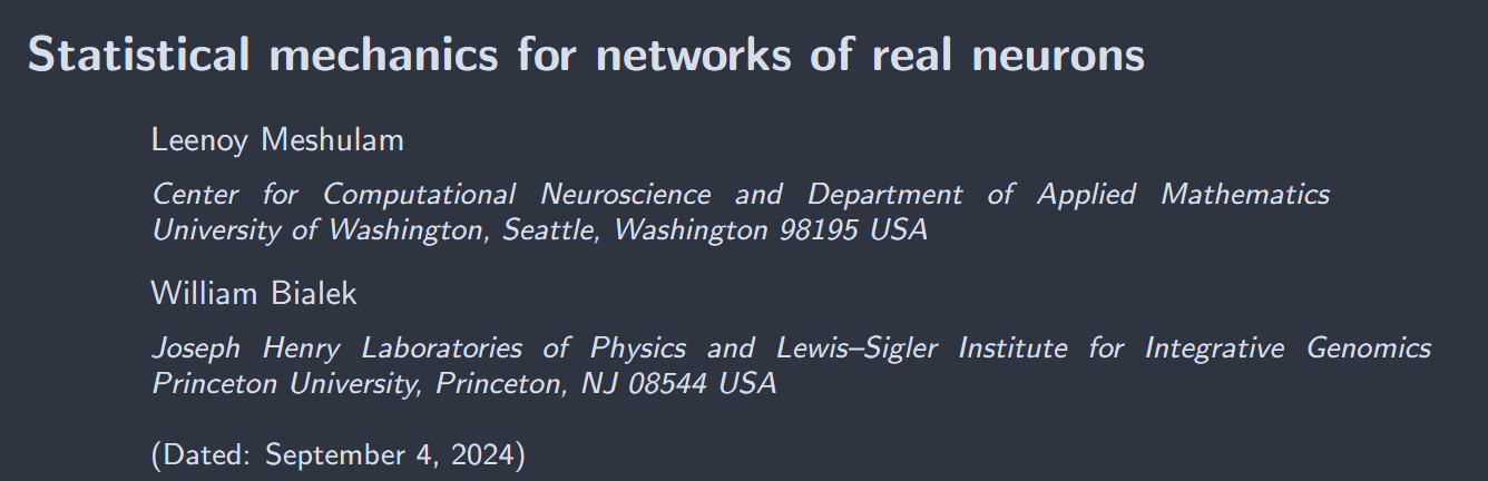
In response to natural movies, the output neurons of the retina—the “ganglion cells” that carry visual signals from eye to brain, and which as a group form the optic nerve—are sparsely activated, generating an average of just a few spikes per second each (Fig 7A, B). Those initial experiments monitored populations of up to forty neurons in a small patch of the retina, with recordings of up to one hour. Pairs of neurons have temporal correlations with a relatively sharp peak or trough on a broad background that tracks longer timescales in the visual input (Fig 7C). If we discretize time into bins of $\Delta\tau = 20$ ms then we capture most of the short time correlations but still have a very low probability of seeing two spikes in the same bin, so that responses of neuron i become binary, $\sigma_{i} = \{0, 1\}$.

为了响应自然活动，视网膜的输出神经元——将视觉信号从眼睛传递到大脑的“神经节细胞”，它们作为一个整体形成视神经——被稀疏激活，每个神经元平均每秒只产生几个尖峰（图 7A，B）。那些初始实验监测了视网膜小块中多达四十个神经元的群体，记录时间长达一小时。成对的神经元具有时间相关性，在视觉输入的较长时间尺度上跟踪较宽背景上的相对尖锐峰值或谷值（图 7C）。如果我们将时间离散化为 $\Delta\tau = 20$ ms 的时间段，那么我们就捕捉到了大部分短时间相关性，但仍然很少看到同一时间段内有两个尖峰，因此神经元 i 的响应变为二进制，$\sigma_{i} = \{0, 1\}$。

FIG. 7 Responses of the salamander retina to naturalistic movies (Schneidman et al., 2006). (A) Raster plot of the action potentials from $N = 40$ neurons. Each dot represents a spike from one cell. (B) Expanded view of the green box in (A), showing the discretization of time into bins of width $\Delta\tau = 20$ms. The result (bottom) is that the state of the network is a binary word $\{\sigma_{i}\}$. (C) Correlations between two neurons. Results are shown as the probability per unit time of a spike in cell $j$ (spike rate) given that there is a spike in cell $i$ at time $t = 0$; the plateau at long times should be the mean rate $r_{j} = \langle\sigma_{j}\rangle/\Delta\tau$. There a peak with a width ~ 100 ms, related to time scales in the visual input, and a peak with width ~ 20ms emphasizes in the inset; this motivates the choice of bins size. (D) Distribution of (off-diagonal) correlation coefficients, from Eq (24), across the population of $N = 40$ neurons. (E) Probability that $K$ out of the $N = 40$ neurons are active in the same time bin (red) compared with expectations if activity of each neuron were independent of all the others (blue). Dashed lines are exponential (red) and Poisson (blue), to guide the eye. (F) Predicted occurrence rates of different binary patterns vs the observed rates, for the independent model $P_{1}$ [Eqs (29, 30), blue] and the pairwise maximum entropy model $P_{2}$ [Eqs (35, 33), red].

图 7 蝾螈视网膜对自然电影的响应（Schneidman 等人，2006）。(A) $N = 40$ 个神经元的动作电位光栅图。每个点代表一个细胞的一个尖峰。(B) (A) 中绿色框的放大视图，显示时间被离散化为宽度为 $\Delta\tau = 20$ms 的时间段。结果（底部）是网络的状态是一个二进制字 $\{\sigma_{i}\}$。(C) 两个神经元之间的相关性。结果显示为在细胞 $i$ 在时间 $t = 0$ 处有一个尖峰的情况下，细胞 $j$ 中尖峰的单位时间概率（尖峰率）；长时间处的平台应该是平均率 $r_{j} = \langle\sigma_{j}\rangle/\Delta\tau$。有一个宽度约为 100 ms 的峰值，与视觉输入中的时间尺度有关，插图中强调了一个宽度约为 20ms 的峰值；这激发了选择箱子大小的动机。(D) 跨越 $N = 40$ 个神经元群体的（非对角线）相关系数的分布，来自方程（24）。(E) 在同一时间段内 $N = 40$ 个神经元中有 $K$ 个活跃的概率（红色）与如果每个神经元的活动独立于所有其他神经元的预期（蓝色）进行比较。虚线分别为指数（红色）和泊松（蓝色），以引导眼睛。(F) 不同二进制模式的预测发生率与观察到的发生率，对于独立模型 $P_{1}$ [方程（29，30），蓝色] 和成对最大熵模型 $P_{2}$ [方程（35，33），红色]。

If we define as usual the fluctuations around the mean,

$$ \delta\sigma_{i} = \sigma_{i} - \langle\sigma_{i}\rangle, $$

then the data sets were large enough to get good estimates of the covariance

$$ C_{ij} = \langle\delta\sigma_{i}\delta\sigma_{j}\rangle = \langle\sigma_{i}\sigma_{j}\rangle_{c} $$

where $\langle\cdots\rangle_{c}$ denotes the connected part of the correlations; in many cases we have more intuition about the correlation matrix

$$ \widetilde{C}_{ij} = \frac{C_{ij}}{\sqrt{C_{ii}C_{jj}}} $$

Importantly, these pairwise correlations are weak: almost all of the $|\widetilde{C}_{i\neq j}|<0.1$, and the bulk of these correlations are just a few percent (Fig 7D). The recordings are long enough that these weak correlations are statistically significant, and almost none of the matrix elements are zero within errors. Correlations thus are weak and widespread, which seems to be common across many different regions of the brain.

如果我们像往常一样定义围绕均值的波动，

$$ \delta\sigma_{i} = \sigma_{i} - \langle\sigma_{i}\rangle, $$

那么数据集足够大，可以很好地估计协方差

$$ C_{ij} = \langle\delta\sigma_{i}\delta\sigma_{j}\rangle = \langle\sigma_{i}\sigma_{j}\rangle_{c} $$

其中 $\langle\cdots\rangle_{c}$ 表示相关性的连接部分；在许多情况下，我们对相关矩阵有更多的直觉

$$ \widetilde{C}_{ij} = \frac{C_{ij}}{\sqrt{C_{ii}C_{jj}}} $$

重要的是，这些成对相关性是弱的：几乎所有的 $|\widetilde{C}_{i\neq j}|<0.1$，而且这些相关性的主体只有几个百分点（图 7D）。记录时间足够长，这些微弱的相关性在统计上是显著的，并且矩阵元素几乎没有在误差范围内为零。因此，相关性是弱而广泛的，这似乎在大脑的许多不同区域中很常见。

If we look just at two neurons, the approximation that they are independent of one another is very good, because the correlations are so weak. But if we look more globally then the widespread correlations combine to have qualitative effects. As an example, we can ask for the probability that $K$ out of $N = 40$ neurons are active in the same time bin, $P_{N}(K)$, and we find that this has a much longer tail than expected if the cells were independent (Fig 7E); simultaneous activity of $K = 10$ neurons already is $\sim 10^{3}\times$ more likely than in the independent model.

如果我们只看两个神经元，由于相关性非常弱，它们相互独立的近似是非常好的。但如果我们更全面地观察，那么广泛的相关性会结合起来产生定性的影响。作为一个例子，我们可以询问在同一时间段内 $N = 40$ 个神经元中有 $K$ 个活跃的概率 $P_{N}(K)$，我们发现如果细胞是独立的，这个概率的尾部要长得多（图 7E）；$K = 10$ 个神经元的同时活动已经比独立模型高出约 $10^{3}$ 倍。

If we focus on $N = 10$ neurons then the experiments are long enough to sample all $\Omega\sim 10^{3}$ states, and the probabilities of these different binary words depart dramatically from the predictions of an independent model (Fig 7F). If we group the different binary words by the total number of active neurons, then the predictions of the independent model actually are anti–correlated with the real data. We emphasize that these failures occur despite the fact that pairwise correlations are weak, and that they are visible at a relatively modest $N = 10$.

如果我们关注 $N = 10$ 个神经元，那么实验时间足够长，可以对所有 $\Omega\sim 10^{3}$ 状态进行采样，并且这些不同二进制字的概率与独立模型的预测有显著偏离（图 7F）。如果我们按活跃神经元的总数对不同的二进制字进行分组，那么独立模型的预测实际上与真实数据呈负相关。我们强调，尽管成对相关性很弱，但这些失败仍然发生，并且它们在相对适度的 $N = 10$ 下是可见的。

If we want to build a model for the patterns of activity in networks of neurons it certainly makes sense to insist that we match the mean activity of each cell. At the risk of being pedantic, what this means explicitly is that we are looking for a probability distribution over network states, $P_{1}(\vec{\sigma})$ that has the maximum entropy while correctly predicting the expectation values

$$ m_{i} \equiv \langle\sigma_{i}\rangle_{\text{expt}} = \langle\sigma_{i}\rangle_{P_{1}} $$

Referring back to Eq (17), the observables that we constrain become

$$ \{f_{\mu}^{(1)}\}\rightarrow \{\sigma_{i}\} $$

note that $i = 1, 2,\cdots, N$, where $N$ is the number of neurons. To implement these constraints we need one Lagrange multiplier for each neuron, and it is convenient to write this multiplier as an “effective field” $h_{i}$, so that the general Eqs (20, 21) become

$$ \begin{aligned} P_{1}(\vec{\sigma}) &= \frac{1}{Z_{1}}\exp{[-E_{1}(\vec{\sigma})]}\\ E_{1}(\vec{\sigma}) &= \sum_{\mu}\lambda_{\mu}^{(1)}f_{\mu}^{(1)}\\ &= \sum_{i=1}^{N}h_{i}\sigma_{i} \end{aligned} $$

We notice that $E_1$ is the energy function for independent spins in local fields, and so the probability distribution over states factorizes,

$$ P_{1}(\vec{\sigma}) \propto \prod_{i=1}^{N}e^{-h_{i}\sigma_{i}} $$

Thus a maximum entropy model which matches only the mean activities of individual neurons is a model in which the activity of each cell is independent of all the others. We have seen that this model is in dramatic disagreement with the data.

如果我们想为神经元网络中的活动模式构建一个模型，坚持匹配每个细胞的平均活动当然是有意义的。冒着啰嗦的风险，这明确意味着我们正在寻找一个网络状态的概率分布 $P_{1}(\vec{\sigma})$，该分布具有最大熵，同时正确预测期望值

$$ m_{i} \equiv \langle\sigma_{i}\rangle_{\text{expt}} = \langle\sigma_{i}\rangle_{P_{1}} $$

回到方程（17），我们约束的可观察量变为

$$ \{f_{\mu}^{(1)}\}\rightarrow \{\sigma_{i}\} $$

注意 $i = 1, 2,\cdots, N$，其中 $N$ 是神经元的数量。为了实现这些约束，我们需要为每个神经元一个拉格朗日乘数，并且将这个乘数写成“有效场” $h_{i}$ 是很方便的，因此一般的方程（20，21）变为

$$ \begin{aligned} P_{1}(\vec{\sigma}) &= \frac{1}{Z_{1}}\exp{[-E_{1}(\vec{\sigma})]}\\ E_{1}(\vec{\sigma}) &= \sum_{\mu}\lambda_{\mu}^{(1)}f_{\mu}^{(1)}\\ &= \sum_{i=1}^{N}h_{i}\sigma_{i} \end{aligned} $$

我们注意到 $E_1$ 是局部场中独立自旋的能量函数，因此状态的概率分布可以分解为，

$$ P_{1}(\vec{\sigma}) \propto \prod_{i=1}^{N}e^{-h_{i}\sigma_{i}} $$

因此，一个仅匹配单个神经元平均活动的最大熵模型是一个每个细胞的活动都独立于所有其他细胞的模型。我们已经看到这个模型与数据有显著的不一致。

A natural first step in trying to capture the nonindependence of neurons is to build a maximum entropy model that matches pairwise correlations. Thus, we are looking for a distribution $P_{2}(\sigma)$ that has maximum entropy while matching the mean activities as in Eq (25) and also the covariance of activity

$$ C_{ij}\equiv \langle\delta\sigma_{i}\delta\sigma_{j}\rangle_{\text{expt}} = \langle\delta\sigma_{i}\delta\sigma_{j}\rangle_{P_{2}} $$

In the language of Eq (17) this means that we have a second set of relevant observables

$$ \{f_{\nu}^{(2)}\} \rightarrow \{\sigma_{i}\sigma_{j}\} $$

As before we need one Lagrange multiplier for each constrained observable, and it is useful to think of the Lagrange multiplier that constrains $\sigma_{i}\sigma_{j}$ as being a “spinspin” coupling $\lambda_{ij} = J_{ij}$. Recalling that each extra constraint adds a term to the effective energy function, Eqs (20, 21) become

$$ \begin{aligned} P_{2}(\vec{\sigma}) &= \frac{1}{Z_{2}(\{h_{i};J_{ij}\})}e^{-E_{2}(\vec{\sigma})}\\ E_{2}(\vec{\sigma}) &= \sum_{\mu}\lambda_{\mu}^{(1)}f_{\mu}^{(1)} + \sum_{\mu}\lambda_{\mu}^{(2)}f_{\mu}^{(2)}\\ &= \sum_{i=1}^{N}h_{i}\sigma_{i} + \frac{1}{2}\sum_{i\neq j}J_{ij}\sigma_{i}\sigma_{j} \end{aligned} $$

This is exactly an Ising model with pairwise interactions among the spins—not an analogy but a mathematical equivalence.

捕捉神经元非独立性的一个自然第一步是构建一个匹配成对相关性的最大熵模型。因此，我们正在寻找一个分布 $P_{2}(\sigma)$，该分布具有最大熵，同时匹配方程（25）中的平均活动以及活动的协方差

$$ C_{ij}\equiv \langle\delta\sigma_{i}\delta\sigma_{j}\rangle_{\text{expt}} = \langle\delta\sigma_{i}\delta\sigma_{j}\rangle_{P_{2}} $$

用方程（17）的语言来说，这意味着我们有第二组相关的可观察量

$$ \{f_{\nu}^{(2)}\} \rightarrow \{\sigma_{i}\sigma_{j}\} $$

像以前一样，我们需要为每个受约束的可观察量一个拉格朗日乘数，并且将约束 $\sigma_{i}\sigma_{j}$ 的拉格朗日乘数视为“自旋-自旋”耦合 $\lambda_{ij} = J_{ij}$ 是有用的。回想一下，每个额外的约束都会向有效能量函数添加一项，方程（20，21）变为

$$ \begin{aligned} P_{2}(\vec{\sigma}) &= \frac{1}{Z_{2}(\{h_{i};J_{ij}\})}e^{-E_{2}(\vec{\sigma})}\\ E_{2}(\vec{\sigma}) &= \sum_{\mu}\lambda_{\mu}^{(1)}f_{\mu}^{(1)} + \sum_{\mu}\lambda_{\mu}^{(2)}f_{\mu}^{(2)}\\ &= \sum_{i=1}^{N}h_{i}\sigma_{i} + \frac{1}{2}\sum_{i\neq j}J_{ij}\sigma_{i}\sigma_{j} \end{aligned} $$

这正是具有自旋之间成对相互作用的 Ising 模型——不是类比，而是数学等价。

Ising models for networks of neurons have a long history, as described in §II.C. In their earliest appearance, these models emerged from a hypothetical, simplified model of the underlying dynamics. Here they emerge as the least structured models consistent with measured properties of the network. As a result, we arrive not at some arbitrary Ising model, where we are free to choose the fields and couplings, but at a particular model that describes the actual network of neurons we are observing. To complete this construction we have to adjust the fields and couplings to match the observed mean activities and correlations. Concretely we have to solve Eqs (25, 31), which can be rewritten as

$$ \begin{aligned} \langle \sigma_{i}\rangle_{\text{expt}} &= \langle\sigma_{i}\rangle_{P_{2}} = \frac{\partial \ln{Z_{2}(\{h_{i};J_{ij}\})}}{\partial h_{i}}\\ \langle\sigma_{i}\sigma_{j}\rangle_{\text{expt}} &= \langle\sigma_{i}\sigma_{j}\rangle_{P_{2}} = \frac{\partial \ln{Z_{2}(\{h_{i};J_{ij}\})}}{\partial J_{ij}} \end{aligned} $$

With $N = 10$ neurons this is challenging but can be done exactly, since the partition function is a sum over just $\Omega\sim 1000$ terms. Once we are done, the model is specified completely. Anything that we compute is a prediction, and there is no room to adjust parameters in search of better agreement with the data.

神经元网络的 Ising 模型有着悠久的历史，如 §II.C 所述。在它们最早出现时，这些模型源自对潜在动力学的假设性简化模型。在这里，它们作为与网络的测量属性一致的最少结构化模型出现。因此，我们不是得到某个任意的 Ising 模型，在那里我们可以自由选择场和耦合，而是得到一个描述我们正在观察的实际神经元网络的特定模型。为了完成这个构建，我们必须调整场和耦合以匹配观察到的平均活动和相关性。具体来说，我们必须解决方程（25，31），它们可以重写为

$$ \begin{aligned} \langle \sigma_{i}\rangle_{\text{expt}} &= \langle\sigma_{i}\rangle_{P_{2}} = \frac{\partial \ln{Z_{2}(\{h_{i};J_{ij}\})}}{\partial h_{i}}\\ \langle\sigma_{i}\sigma_{j}\rangle_{\text{expt}} &= \langle\sigma_{i}\sigma_{j}\rangle_{P_{2}} = \frac{\partial \ln{Z_{2}(\{h_{i};J_{ij}\})}}{\partial J_{ij}} \end{aligned} $$

对于 $N = 10$ 个神经元来说，这具有挑战性，但可以精确完成，因为配分函数只是 $\Omega\sim 1000$ 项的总和。一旦我们完成，模型就完全指定了。我们计算的任何东西都是一个预测，没有调整参数以寻求与数据更好一致的余地。

As noted above, with $N = 10$ neurons the experiments are long enough to get a reasonably full sampling of the probability distribution over $\vec{\sigma}$. This provides the most detailed possible test of the model $P_{2}$, and in Fig 7F we see that the agreement between theory and experiment is excellent, except for very rare patterns where errors in the estimate of the probability are larger. Similar results are obtained for other groups of $N = 10$ cells drawn out of the full population of $N = 40$. Quantitatively we can measure the Jensen–Shannon divergence between the estimated distribution $P_{\text{data}}(\sigma)$ and the model $P_{2}(\sigma)$; across multiple choices of ten cells this fluctuates by a factor of two around $D_{JS} = 0.001$ bits, which means that it takes thousands of independent observations to distinguish the model from the data.

正如上面所指出的，对于 $N = 10$ 个神经元，实验时间足够长，可以对 $\vec{\sigma}$ 上的概率分布进行合理完整的采样。这为模型 $P_{2}$ 提供了最详细的可能测试，在图 7F 中我们看到理论与实验之间的一致性非常好，除了非常罕见的模式，其中概率估计的误差较大。从完整的 $N = 40$ 群体中抽取的其他 $N = 10$ 个细胞组也得到了类似的结果。我们可以定量地测量估计分布 $P_{\text{data}}(\sigma)$ 与模型 $P_{2}(\sigma)$ 之间的 Jensen–Shannon 散度；在多个十个细胞的选择中，这个值围绕 $D_{JS} = 0.001$ 比特波动了两倍，这意味着需要数千次独立观察才能区分模型与数据。

The architecture of the retina is such that many individual output neurons can be driven or inhibited by a single common neuron that is internal to the circuitry. This is one of many reasons that one might expect significant combinatorial regulation in the patterns of activity, and there were serious efforts to search for these effects (Schnitzer and Meister, 2003). The success of a pairwise model thus came as a considerable surprise.

视网膜的结构使得许多个体输出神经元可以被电路内部的单个共同神经元驱动或抑制。这是许多原因之一，人们可能会期望在活动模式中存在显著的组合调节，并且曾经有认真努力去寻找这些效应（Schnitzer 和 Meister，2003）。因此，成对模型的成功令人相当惊讶。

The results in the salamander retina, with natural inputs, were quickly confirmed in the primate retina using simpler inputs (Shlens et al., 2006). Those experiments covered a larger area and thus could focus on sub–populations of neurons belonging to a single class, which are arrayed in a relatively regular lattice. In this case not only did the pairwise model work very well, but the effective interactions $J_{ij}$ were confined largely to nearest neighbors on this lattice.

蝾螈视网膜中使用自然输入的结果很快在灵长类动物视网膜中得到了确认，使用了更简单的输入（Shlens 等人，2006）。这些实验覆盖了更大的区域，因此可以专注于属于单一类别的神经元亚群，这些神经元排列在一个相对规则的晶格中。在这种情况下，不仅成对模型效果非常好，而且有效相互作用 $J_{ij}$ 主要局限于该晶格上的最近邻。

Pairwise maximum entropy models also were reasonably successful in describing patterns of activity across $N\leq 10$ neurons sampled from a cluster of cortical neurons kept alive in a dish (Tang et al., 2008). This work also pointed to the fact that dynamics did not correspond to Brownian motion on the energy surface.

成对最大熵模型在描述从培养皿中保持活力的一簇皮层神经元中采样的 $N\leq 10$ 个神经元的活动模式方面也相当成功（Tang 等人，2008）。这项工作还指出，动力学并不对应于能量表面上的布朗运动。

These early successes with small numbers of neurons raised many questions. For example, the interaction matrix $J_{ij}$ contained a mix of positive and negative terms, suggesting that frustration could lead to many local minima of the energy function or equivalently local maxima of the probability $P(\vec{\sigma})$, as in the Hopfield model (§II.C); could these “attractors” have a function in representing the visual world? Relatedly, an important consequence of the collective behavior in the Ising model is that if we know that state of all neurons in the network but one, then we have a parameter–free prediction for the probability that this last neuron will be active; does this allow for error correction? To address these and other issues one must go beyond $N\sim 10$ cells, which was already possible experimentally. But at larger $N$ one needs more powerful methods for solving the inverse problem that is at the heart of the maximum entropy construction, as described in Appendix B.

这些早期在少量神经元上的成功引发了许多问题。例如，交互矩阵 $J_{ij}$ 包含正负混合项，表明阻挫可能导致能量函数的许多局部极小值，或者等价地，概率 $P(\vec{\sigma})$ 的局部极大值，就像 Hopfield 模型（§II.C）中一样；这些“吸引子”在表示视觉世界方面是否具有功能？相关地，Ising 模型中集体行为的一个重要后果是，如果我们知道网络中除一个神经元外所有神经元的状态，那么我们就可以无参数地预测这个最后一个神经元是否会活跃；这是否允许纠错？为了处理这些和其他问题，必须超越 $N\sim 10$ 个细胞，这在实验上已经是可能的。但在更大的 $N$ 下，需要更强大的方法来解决最大熵构造核心的逆问题，如附录 B 所述。

The equivalence to equilibrium models entices us to describe the couplings $J_{ij}$ as “interactions,” but there is no reason to think that these correspond to genuine connections between cells. In particular, $J_{ij}$ is symmetric because it is an effective interaction driving the equaltime correlations of activity in cells $i$ and $j$, and these correlations are symmetric by definition. If we go beyond single time slices to describe trajectories of activity over time, then with multiple cells the effective interactions can become asymmetric and break timereversal invariance.

与平衡模型的等价性诱使我们将耦合 $J_{ij}$ 描述为“相互作用”，但没有理由认为它们对应于细胞之间的真正连接。特别是，$J_{ij}$ 是对称的，因为它是驱动细胞 $i$ 和 $j$ 活动的同时相关性的有效相互作用，而这些相关性按定义是对称的。如果我们超越单个时间片来描述随时间变化的活动轨迹，那么对于多个细胞，有效相互作用可以变得不对称并打破时间反演不变性。

Before leaving the early work, it is useful to step back and ask about the goals and hopes from that time. As reviewed above, the use of statistical physics models for neural networks has a deep history. Saying that the brain is described by an Ising model captured both the optimism and (one must admit) the naı ̈vet ́e of the physics community in approaching the phenomena of life. One could balance optimism and naı ̈vet ́e by retreating to the position that these models are metaphors, illustrating what could happen rather than being theories of what actually happens. The success of maximum entropy models in the retina gave an example of how statistical physics ideas could provide a quantitative theory for networks of real neurons.

在离开早期工作之前，退一步问一下当时的目标和希望是有用的。如上所述，神经网络使用统计物理模型有着深厚的历史。说大脑由 Ising 模型描述既捕捉了乐观主义，也捕捉了（必须承认）物理学界在接近生命现象时的天真。通过退回到这些模型是隐喻的位置，可以平衡乐观主义和天真，说明可能会发生什么，而不是实际发生的理论。视网膜中最大熵模型的成功提供了一个例子，说明统计物理思想如何为真实神经元网络提供定量理论。

Larger networks of neurons

The use of maximum entropy for networks of real neurons quickly triggered almost all possible reactions: (a) It should never work, because systems are not in equilibrium, have combinational interactions, $\cdots$ . (b) It could work, but only under uninteresting conditions. (c) It should always work, since these models are very expressive. (d) It works at small $N$ , but this is a poor guide to what will happen at large $N$ . (e) Sure, but why not use [favorite alternative], for which we have efficient algorithms?

对于真实神经元网络使用最大熵迅速引发了几乎所有可能的反应：（a）它永远不会起作用，因为系统不处于平衡状态，具有组合相互作用，$\cdots$（b）它可能起作用，但仅在无趣的条件下。（c）它应该总是有效，因为这些模型非常有表现力。（d）它在小 $N$ 下有效，但这对大 $N$ 会发生什么没有很好的指导意义。（e）当然，但为什么不使用[最喜欢的替代方案]，我们有高效的算法？

Perhaps the most concrete response to these issues is just to see what happens as we move to more examples, especially in larger networks. But we should do this with several questions in mind, some of which were very explicit in the early literature (Macke et al., 2011a; Roudi et al., 2009). First, finding the maximum entropy model that matches the desired constraints—that is, solving Eqs (17)—becomes more difficult at larger $N$ . Can we be sure that we are testing the maximum entropy idea, and our choice of constraints, rather than the efficacy of our algorithms for solving this problem?

也许对这些问题最具体的回应就是看看当我们转向更多例子，特别是在更大网络中会发生什么。但我们应该牢记几个问题，其中一些在早期文献中非常明确（Macke 等人，2011a；Roudi 等人，2009）。首先，找到匹配所需约束的最大熵模型——即解决方程（17）——在更大的 $N$ 下变得更加困难。我们能否确定我们正在测试最大熵的想法，以及我们选择的约束，而不是我们解决这个问题的算法的有效性？

Second, as N increases the maximum entropy construction becomes very data hungry. This concern often is phrased as the usual problem of “over–fitting,” when the number of parameters in our model is too large to fully constrained by the data. But in the maximum entropy formulation the problem is even more fundamental. The maximum entropy construction builds the least structured model consistent with a set of known expectation values. With a finite amount of data, if our list of expectation values is too long then the claim that we “know” these features of the system just isn’t true, and this problem arises even before we try to build the maximum entropy model.

其次，随着 N 的增加，最大熵构造变得非常需要数据。这个问题通常被表述为“过拟合”的常见问题，当我们模型中的参数数量太大而无法被数据完全约束时。但在最大熵公式中，这个问题甚至更为根本。最大熵构造建立了一个与一组已知期望值一致的最少结构化模型。对于有限的数据量，如果我们的期望值列表太长，那么我们“知道”系统的这些特征的说法就不是真的，即使在我们尝试构建最大熵模型之前，这个问题也会出现。

Third, because correlations are spread widely in these networks, if one develops a perturbation theory around the limit of independent neurons then factors of $N$ appear in the series, e.g. for the entropy per neuron. Success at modest $N$ might thus mean that we are in a perturbative regime, which would be much less interesting. The question of whether success is perturbative is subtle, since at finite $N$ all properties of the maximum entropy model are analytic functions of the correlations, and hence if we carry perturbation theory far enough we will get the right answer (Sessak and Monasson, 2009).

第三，因为相关性在这些网络中广泛传播，如果我们围绕独立神经元的极限发展微扰理论，那么 $N$ 的因素会出现在级数中，例如每个神经元的熵。因此，在适度的 $N$ 下的成功可能意味着我们处于微扰范围内，这将不那么有趣。成功是否是微扰的问题是微妙的，因为在有限的 $N$ 下，最大熵模型的所有属性都是相关性的解析函数，因此如果我们将微扰理论进行得足够远，我们将得到正确的答案（Sessak 和 Monasson，2009）。

Finally, in statistical mechanics we are used to the idea of a large $N$, thermodynamic limit. Although this carries over to model networks (Amit, 1989), it is not obvious how to use this idea in thinking about networks of real neurons. Naive extrapolation of results from maximum entropy models of $N = 10 − 20$ neurons in the retina indicated that something special had to happen by $N\sim 200$, or else the entropy would vanish; this was interesting because $N\sim 200$ is the number cells that are “looking” at overlapping regions of the visual world (Schneidman et al., 2006). A more sophisticated extrapolation imagines a large population of neurons in which mean activities and pairwise correlations are drawn at random from the same distribution as found in recordings from smaller numbers of neurons (Tkaˇcik et al., 2006, 2009). This sort of extrapolation is motivated in part by the observation that “thermodynamic” properties of the maximum entropy models learned for $N = 20$ or $N = 40$ retinal neurons match the behavior of such random models at the same $N$. If we now extrapolate to $N = 120$ there are striking collective behaviors, and we will ask if these are seen in real data from $N > 100$ cells.

最后，在统计力学中，我们习惯于大 $N$、热力学极限的概念。尽管这可以转移到模型网络中（Amit，1989），但在思考真实神经元网络时如何使用这个想法并不明显。从视网膜中 $N = 10 − 20$ 个神经元的最大熵模型结果的天真外推表明，到 $N\sim 200$ 时必须发生一些特殊的事情，否则熵将消失；这是有趣的，因为 $N\sim 200$ 是“观察”视觉世界重叠区域的细胞数量（Schneidman 等人，2006）。更复杂的外推设想了一个大型神经元群体，其中平均活动和成对相关性是从与较少神经元记录中发现的相同分布中随机抽取的（Tkaˇcik 等人，2006，2009）。这种外推部分是由观察到为 $N = 20$ 或 $N = 40$ 视网膜神经元学习的最大熵模型的“热力学”属性与同一 $N$ 下此类随机模型的行为相匹配所激发的。如果我们现在外推到 $N = 120$，会出现显著的集体行为，我们将询问在来自 $N > 100$ 个细胞的真实数据中是否看到了这些行为。

Early experiments in the retina already were monitoring $N = 40$ cells, and the development of numerical methods described in Appendix B quickly allowed analysis of these larger data sets (Tkaˇcik et al., 2006, 2009). With $N = 40$ cells one cannot check the predictions for probabilities of individual patterns $P(\vec{\sigma})$, but one can check the probability that $K$ out of $N$ cells are active in the same small time bin, as in Fig. 7E, or the correlations among triplets of neurons. At $N = 40$ we see the first hints that constraining pairwise correlations is not quite enough to capture the full structure of the network. There are disagreements between theory and experiment in the tails of the distribution $P_{N}(K)$, and more importantly a few percent disagreement at $K = 0$. This may not seem like much, but since the network is completely silent in roughly half of the $\Delta\tau = 20$ ms time bins, the data determine $P_{N}(K = 0)$ very precisely, and a one percent discrepancy is hugely significant.

视网膜中的早期实验已经监测了 $N = 40$ 个细胞，并且附录 B 中描述的数值方法的发展很快允许分析这些更大的数据集（Tkaˇcik 等人，2006，2009）。对于 $N = 40$ 个细胞，我们无法检查单个模式 $P(\vec{\sigma})$ 概率的预测，但我们可以检查在同一小时间段内 $N$ 个细胞中有 $K$ 个活跃的概率，如图 7E 所示，或神经元三元组之间的相关性。在 $N = 40$ 时，我们看到了一些迹象表明，仅约束成对相关性还不足以捕捉网络的完整结构。分布 $P_{N}(K)$ 的尾部存在理论与实验之间的不一致，更重要的是在 $K = 0$ 处存在几个百分点的不一致。这似乎不多，但由于网络在大约一半的 $\Delta\tau = 20$ 毫秒时间段内完全静默，数据非常精确地确定了 $P_{N}(K = 0)$，而且百分之一的差异是非常显著的。

A new generation of electrode arrays made it possible to record $N = 100 − 200$ cells, densely sampling a small patch of the retina (§III.A). As an example, these experiments could capture the signals from $N_{\text{max}} = 160$ ganglion cells in a $(450 \mu\text{m})^2$ area of the salamander retina that contains a total of $N\sim 200$ cells, and these recordings are stable for $\sim 1.5$ hr.

新一代电极阵列使得记录 $N = 100 − 200$ 个细胞成为可能，密集采样视网膜的小块（§III.A）。作为一个例子，这些实验可以捕捉到来自蝾螈视网膜中 $(450 \mu\text{m})^2$ 区域的 $N_{\text{max}} = 160$ 个神经节细胞的信号，该区域总共有 $N\sim 200$ 个细胞，并且这些记录在 $\sim 1.5$ 小时内是稳定的。

As explained in Appendix B, we can build maximum entropy models at larger $N$ by using Monte Carlo simulation to estimate expectation values in the model, comparing with the measured expectation values, and then adjusting the coupling constants to improve the agreement. Necessarily this doesn’t yield an exact solution to the constraint Eqs (17), but this seems acceptable since we are trying to match expectation values that are estimated from experiment and these have errors. Figure 8A shows that with $N = 100$ we can match the observed pairwise correlations within experimental error (Tkaˇcik et al., 2014). More precisely the errors in predicting the elements of the covariance matrix $C_{ij}$ [Eq (23)] are nearly Gaussian, with a variance equal to the variance of the measurement errors. This suggests, strongly, that one can successfully fit, but not over–fit, a maximum entropy model to these data.

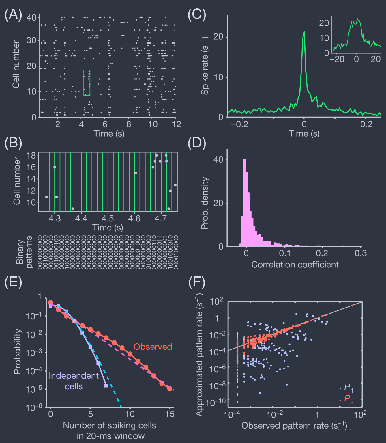
如附录 B 所述，我们可以通过使用蒙特卡罗模拟来估计模型中的期望值，将其与测量的期望值进行比较，然后调整耦合常数以改善一致性，从而在更大的 $N$ 下构建最大熵模型。必然地，这不会产生对约束方程（17）的精确解，但这似乎是可以接受的，因为我们正在尝试匹配从实验中估计的期望值，而这些期望值存在误差。图 8A 显示，在 $N = 100$ 时，我们可以在实验误差范围内匹配观察到的成对相关性（Tkaˇcik 等人，2014）。更准确地说，预测协方差矩阵 $C_{ij}$ [方程（23）] 元素的误差几乎是高斯分布的，其方差等于测量误差的方差。这强烈表明，可以成功地拟合，但不会过拟合这些数据的最大熵模型。

FIG. 8 Fitting, but not over-fitting, with $N\sim 100$ neurons (Tkaéik et al., 2014). (A) Distribution of errors in the prediction of pairwise correlations, after adjusting the parameters $\{h_{i}; J_{ij}\}$, for $N = 100$. Prediction errors are in units of the measurement error $\Delta C_{ij}$ for each element of the covariance matrix. Red line shows a Gaussian with zero mean and unit variance. (B) Log—likelihood [Eq (38)] of test data not used in constructing the maximum entropy model, in units of the result for the training data. At $N = 10$ it is not surprising that these agree, since the number of parameters $\{h_{i}; J_{ij}\}$ is small. But we see this agreement persists at the $\sim 1%$ level out to $N = 120$, showing that even models for relatively large networks are not overfit.

图 8 使用 $N\sim 100$ 个神经元进行拟合，但没有过拟合（Tkaéik 等人，2014）。（A）在调整参数 $\{h_{i}; J_{ij}\}$ 后，对于 $N = 100$，预测成对相关性的误差分布。预测误差以协方差矩阵每个元素的测量误差 $\Delta C_{ij}$ 为单位。红线显示了均值为零、方差为一的高斯分布。（B）测试数据的对数似然 [方程（38）]，以训练数据结果为单位。在 $N = 10$ 时，这些结果一致并不令人惊讶，因为参数数量 $\{h_{i}; J_{ij}\}$ 很少。但我们看到这种一致性在 $N = 120$ 时仍然保持在约 $1%$ 的水平，表明即使是相对较大网络的模型也没有过拟合。

The test for fitting vs over–fitting in Fig 8A looks at each pair of cells individually, but part of the worry is that at large N we can have accurate estimates of individual elements Cij while under–determining the global properties of the matrix. We can take a familiar empirical approach, measuring the means ⟨σi⟩ and covariances ⟨δσiδσj⟩c in 90% of the data, using these to infer the parameters {hi; Jij} in a maximum entropy model, and then testing the predictions of the model [Eqs (35, 33)] on the remaining 10%. The fundamental measure of model quality is the log–likelihood of the data, which we can normalize per sample and per neuron

$$ \mathcal{L} = \frac{1}{N}\langle \log{P(\vec{\sigma})}\rangle_{\text{expt}} $$

Figure 8B shows that $\mathcal{L}$ is the same, to better than one percent, whether we evaluate it over the training data or over the test data. This is true at $N = 10$, where surely there can be no question that we have enough samples, and it is true at $N = 120$.

拟合与过拟合的测试如图 8A 所示，单独查看每对细胞，但部分担忧是，在大 N 下，我们可以准确估计单个元素 Cij，同时未确定矩阵的全局属性。我们可以采用熟悉的经验方法，在 90% 的数据中测量均值 ⟨σi⟩ 和协方差 ⟨δσiδσj⟩c，使用这些来推断最大熵模型中的参数 {hi; Jij}，然后在剩余的 10% 上测试模型的预测 [方程（35，33）]。模型质量的基本度量是数据的对数似然，我们可以按样本和每个神经元进行归一化

$$ \mathcal{L} = \frac{1}{N}\langle \log{P(\vec{\sigma})}\rangle_{\text{expt}} $$

图 8B 显示，无论我们是在训练数据上还是在测试数据上评估 $\mathcal{L}$，其值都相同，误差小于百分之一。这在 $N = 10$ 时是真的，在那里肯定没有问题，我们有足够的样本，并且在 $N = 120$ 时也是真的。

Different networks of neurons, in different organisms and different regions of the brain, have different correlation structures. One should thus be wary of generalizations such as “an hour is enough data for one hundred neurons.” But at least in the context of experiments on the retina, there is no question that maximum entropy models can be learned reliably from the available data, and that there is no over–fitting. Said another way, the models really are the solutions to the mathematical problem that we set out to solve (§IV.A): What is the minimal model consistent with a set of expectation values measured in experiment? These models do not carry signatures of the algorithm that we used to find them, nor are they systematically perturbed by the finiteness of the data on which they are based. This answers the first two questions formulated above.

不同生物体和大脑不同区域的神经元网络具有不同的相关结构。因此，人们应该对“一小时足够一百个神经元的数据”之类的概括持谨慎态度。但至少在视网膜实验的背景下，毫无疑问，最大熵模型可以从可用数据中可靠地学习，并且没有过拟合。换句话说，这些模型确实是我们着手解决的数学问题的解决方案（§IV.A）：与实验中测量的一组期望值一致的最小模型是什么？这些模型不携带我们用来找到它们的算法的特征，也不会被它们所基于的数据的有限性系统地扰动。这回答了上面提出的前两个问题。

Given that we can construct the maximum entropy models reliably, what do we learn? To begin, the small discrepancies in predicting the probability that $K$ out $N$ neurons are active simultaneously, $P_{N}(K)$, become larger as $N$ increases. The simplest solution to this problem is to add one more constraint, insisting that the maximum entropy model match the observed $P_{N}(K)$ exactly. This adds only $\sim N$ constraints to a problem in which we already have $N(N + 1)/2$, so the resulting “$K$–pairwise” models are not significantly more complex.

鉴于我们可以可靠地构建最大熵模型，我们学到了什么？首先，预测 $K$ 个神经元同时活跃的概率 $P_{N}(K)$ 时的小差异随着 $N$ 的增加而变大。解决这个问题的最简单方法是添加一个额外的约束，坚持让最大熵模型准确匹配观察到的 $P_{N}(K)$。这在我们已经有 $N(N + 1)/2$ 个约束的问题中只增加了 $\sim N$ 个约束，因此得到的“$K$–成对”模型并没有显著更复杂。

Again, at the risk of being pedantic let’s formulate matching of the observed $P_{N}(K)$ as constraining expectation values. If we introduce the Kronecker delta for integers $n$ and $m$,

$$ \begin{aligned} \delta &= 1\quad n=m\\ &= 0\quad n\neq m \end{aligned} $$

then

$$ P_{N}(K) = \left\langle \delta\left( K,\sum_{i}^{N}\sigma_{i} \right)\right\rangle $$

Thus to match $P_{N}(K)$ we want to enlarge our set of observables to include

$$ \{f_{\mu}^{(\text{counts})}\} \rightarrow \left\{\delta\left(K,\sum_{i}^{N}\sigma_{i}\right)\right\} $$

As before, each new constraint adds a term to the effective energy,

$$ E(\vec{\sigma}) = \sum_{\mu}\lambda_{\mu}^{(\text{counts})}f_{\mu}^{(\text{counts})} = \sum_{K=0}^{N}\lambda_{K}\delta\left(K, \sum_{i}^{N}\sigma_{i}\right) $$

It is useful to think of this as an effective potential that acts on the summed activity,

$$ \sum_{K=0}^{N}\lambda_{K}\delta\left(K,\sum_{i}^{N}\sigma_{i}\right) = V\left(\sum_{i=1}^{N}\sigma_{i}\right) $$

再次，为了避免过于迂腐，让我们将匹配观察到的 $P_{N}(K)$ 表述为约束期望值。如果我们引入整数 $n$ 和 $m$ 的 Kronecker delta，

$$ \begin{aligned} \delta &= 1\quad n=m\\ &= 0\quad n\neq m \end{aligned} $$

那么

$$ P_{N}(K) = \left\langle \delta\left( K,\sum_{i}^{N}\sigma_{i} \right)\right\rangle $$

因此，为了匹配 $P_{N}(K)$，我们希望将我们的可观察量集合扩大到包括

$$ \{f_{\mu}^{(\text{counts})}\} \rightarrow \left\{\delta\left(K,\sum_{i}^{N}\sigma_{i}\right)\right\} $$

如前所述，每个新约束都会向有效能量添加一项，

$$ E(\vec{\sigma}) = \sum_{\mu}\lambda_{\mu}^{(\text{counts})}f_{\mu}^{(\text{counts})} = \sum_{K=0}^{N}\lambda_{K}\delta\left(K, \sum_{i}^{N}\sigma_{i}\right) $$

将其视为作用于总活动的有效势是有用的，

$$ \sum_{K=0}^{N}\lambda_{K}\delta\left(K,\sum_{i}^{N}\sigma_{i}\right) = V\left(\sum_{i=1}^{N}\sigma_{i}\right) $$

Putting the pieces together, the maximum entropy model that matches the mean activity of individual neurons, the correlations between pairs of neurons, and the probability that $K$ out of $N$ are active simultaneously takes the form

$$ \begin{aligned} P_{2k}(\vec{\sigma}) &= \frac{1}{Z_{2k}}e^{-E_{2k}(\vec{\sigma})}\\ E_{2k}(\vec{\sigma}) &= \sum_{i=1}^{N}h_{i}\sigma_{i} + \frac{1}{2}\sum_{i\neq j}J_{ij}\sigma_{i}\sigma_{j} + V\left(\sum_{i=1}^{N}\sigma_{i}\right) \end{aligned} $$

We refer to this as the “$K$–pairwise” model (Tkaˇcik et al., 2014).

将各个部分组合在一起，匹配单个神经元的平均活动、神经元对之间的相关性以及 $N$ 个中有 $K$ 个同时活跃的概率的最大熵模型形式为

$$ \begin{aligned} P_{2k}(\vec{\sigma}) &= \frac{1}{Z_{2k}}e^{-E_{2k}(\vec{\sigma})}\\ E_{2k}(\vec{\sigma}) &= \sum_{i=1}^{N}h_{i}\sigma_{i} + \frac{1}{2}\sum_{i\neq j}J_{ij}\sigma_{i}\sigma_{j} + V\left(\sum_{i=1}^{N}\sigma_{i}\right) \end{aligned} $$

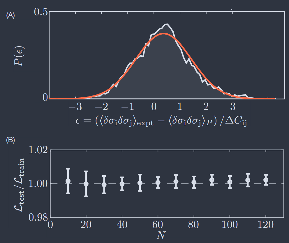
We can test this model immediately by estimating the correlations among triplets of neurons,

$$ C_{ijk} = \langle (\sigma_{i}-\langle\sigma_{i}\rangle)(\sigma_{j}-\langle\sigma_{j}\rangle)(\sigma_{k}-\langle\sigma_{k}\rangle)\rangle $$

Figure 9 shows the results with averages computed in both the pairwise and K–pairwise models, plotted vs. the experimental values. The discrepancies are very small, although still roughly three times larger than the experimental errors in the estimates of the correlations themselves (Tkacˇik et al., 2014); we will see that one can sometimes get even better agreement (§V). Note that the potential $V$ which we add to match the constraint on $P_{N}(K)$ does not carry any information about the identities of the individual neurons. It thus is interesting that including this term improves the prediction of all the triplet correlations, which do depend on neural identity.

我们可以通过估计神经元三元组之间的相关性来立即测试这个模型，

$$ C_{ijk} = \langle (\sigma_{i}-\langle\sigma_{i}\rangle)(\sigma_{j}-\langle\sigma_{j}\rangle)(\sigma_{k}-\langle\sigma_{k}\rangle)\rangle $$

图 9 显示了在成对和 K–成对模型中计算的平均值与实验值的结果。尽管与相关性本身估计的实验误差相比仍然大约大三倍，但差异非常小（Tkacˇik 等人，2014）；我们将看到有时可以获得更好的结果（§V）。请注意，我们添加以匹配 $P_{N}(K)$ 约束的势 $V$ 不包含有关单个神经元身份的任何信息。因此，值得注意的是，包括这一项改善了对所有三元组相关性的预测，而这些相关性确实取决于神经元的身份。

Triplet correlations for $N = 100$ cells in the retina (Tkaˇcik et al., 2014). Measured $C_{ijk}$ (x-axis) vs predicted by the model (y-axis), shown for a single subgroup. The $\sim 1.6 \times 10^{5}$ distinct triplets are grouped into 1000 equally populated bins; error bars in x are s.d. across the bin. The corresponding values for the predictions are grouped together, yielding the mean and the s.d. of the prediction (y-axis). Inset zooms in on the bulk of the predictions at small correlation, for the $K$–pairwise model. The original reference used $\sigma_{i} = \pm 1$, so that all the $C_{ijk}$ shown here are $8\times$ larger than they would be in the $\sigma_{i} = {0, 1}$ representation.

图 9 视网膜中 $N = 100$ 个细胞的三元组相关性（Tkaˇcik 等人，2014）。测量的 $C_{ijk}$（x 轴）与模型预测的值（y 轴），显示为单个子组。大约 $1.6 \times 10^{5}$ 个不同的三元组被分成 1000 个同等人口的箱；x 轴上的误差条是跨箱的标准差。预测的相应值被分组在一起，产生预测的均值和标准差（y 轴）。插图放大了 $K$–成对模型中小相关性的预测主体。原始参考使用 $\sigma_{i} = \pm 1$，因此这里显示的所有 $C_{ijk}$ 都比 $\sigma_{i} = {0, 1}$ 表示法中的值大 $8\times$。

With $N = 100$ cells we cannot check, as in Fig 7F, the probability of every state of the network. But the model assigns to every state an energy $E_{2k}(\vec{\sigma})$, and we can ask about the distribution of this energy over the states that we see in the experiment vs. the expectation if states are drawn out of the model. To emphasize the extremes we look at the high energy tail,

$$ \Phi(E) = \langle\Theta[E - E_{2k}(\vec{\sigma})]\rangle $$

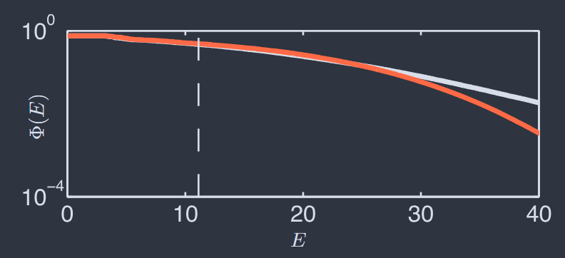
where $\Theta(x)$ is the unit step function and the expectation value can be taken over the data or the theory. Figure 10 shows the comparison between theory and experiment. Note that the plot extends far past the point where individual states are predicted to occur once over the duration of the experiment, but we can make meaningful statements in this regime because there are (exponentially) many such states. Close agreement between theory and experiment extends out to $E\sim 25$, corresponding to states that are predicted to occur roughly once per fifty years.

对于 $N = 100$ 个细胞，我们无法像图 7F 那样检查网络每个状态的概率。但模型为每个状态分配了一个能量 $E_{2k}(\vec{\sigma})$，我们可以询问实验中看到的状态的能量分布与从模型中抽取状态时的期望值。为了强调极端情况，我们查看高能尾部，

$$ \Phi(E) = \langle\Theta[E - E_{2k}(\vec{\sigma})]\rangle $$

其中 $\Theta(x)$ 是单位阶跃函数，期望值可以在数据或理论上进行。图 10 显示了理论与实验之间的比较。请注意，该图远远超出了预测在实验持续时间内单独状态出现一次的点，但我们可以在这个范围内做出有意义的陈述，因为存在（指数级）许多这样的状态。理论与实验之间的密切一致延伸到 $E\sim 25$，对应于大约每五十年预测出现一次的状态。

FIG. 10 The cumulative distribution of energies for $N = 120$ neurons (Tkacˇik et al., 2014). $\Phi(E)$ is defined in Eq (48), and averages are over data (black) or the theory (red). Dashed vertical line denotes an energy $E_{2k}(\sigma)$ such that the particular state $\sigma$ should occur on average once during the duration of the experiment.

图 10 $N = 120$ 个神经元的能量累积分布（Tkacˇik 等人，2014）。$\Phi(E)$ 在方程（48）中定义，平均值是基于数据（黑色）或理论（红色）。虚线垂直线表示能量 $E_{2k}(\sigma)$，使得特定状态 $\sigma$ 在实验持续时间内平均出现一次。

This class of models predicts that neural activity is collective. Thus in a population of $N$ cells, if we know the state of $N −1$ we can make a prediction of the probability that the last cell will be active,

$$ P(\sigma_{i}=1|\{\sigma_{i\neq j}\}) = \frac{1}{1 + \exp{[-h_{i}^{\text{eff}}(\{\sigma_{i\neq j}\})]}} $$

where we can think of the other neurons as applying an effective field to the one neuron that we focus on,

$$ \begin{aligned} h_{i}^{\text{eff}}(\{\sigma_{i\neq j}\}) = &E(\sigma_{1},\sigma_{2},\cdots,\sigma_{i}=1,\cdots,\sigma_{N}) \\ -&E(\sigma_{1},\sigma_{2},\cdots,\sigma_{i}=0,\cdots,\sigma_{N}) \end{aligned} $$

For each neuron and for each moment in time we can calculate the effective field predicted by the theory, with no free parameters, and we can group together all instances in which this field is in some narrow range and ask if the probability of the cell being active agrees with Eq (B8). Results are shown in Fig. 11A.

这种模型类预测神经活动是集体的。因此，在 $N$ 个细胞的群体中，如果我们知道 $N −1$ 的状态，我们可以预测最后一个细胞活跃的概率，

$$ P(\sigma_{i}=1|\{\sigma_{i\neq j}\}) = \frac{1}{1 + \exp{[-h_{i}^{\text{eff}}(\{\sigma_{i\neq j}\})]}} $$

其中我们可以将其他神经元视为对我们关注的一个神经元施加有效场，

$$ \begin{aligned} h_{i}^{\text{eff}}(\{\sigma_{i\neq j}\}) = &E(\sigma_{1},\sigma_{2},\cdots,\sigma_{i}=1,\cdots,\sigma_{N}) \\ -&E(\sigma_{1},\sigma_{2},\cdots,\sigma_{i}=0,\cdots,\sigma_{N}) \end{aligned} $$

对于每个神经元和每个时间点，我们都可以计算理论预测的有效场，没有自由参数，并且我们可以将所有实例分组在一起，其中该场处于某个狭窄范围内，并询问细胞活跃的概率是否与方程（B8）一致。结果如图 11A 所示。

FIG. 11 Effective fields and the collective character of neural activity in the retina (Tkacˇik et al., 2014). (A) The probability that a single neuron is active given the state of the rest of the network, with $N = 120$. Points with error bars are the data, with the effective field computed from the model as in Eq (50). Red line is the prediction from Eq (49), and grey points are results with the purely pairwise rather than “$K$–pairwise” model. Shaded grey region shows the distribution of fields across the experiment, emphasizing that the errors at large positive field are in the tail of the distribution. Inset shows the same results on a logarithmic scale for probability. (B) Probability of a single neuron being active as a function of time in a repeated naturalistic movie, normalized as the probability per unit time of an action potential (spikes/s). Top, in red, experimental data. Lower traces, in black, predictions based on states of other neurons in an $N$–cell group, based on Eqs (B8, 50). Solid lines are the mean prediction across all repetitions of the movie, and thin lines are the envelope $\pm$ one standard deviation.

图 11 视网膜中神经活动的有效场和集体特征（Tkacˇik 等人，2014）。（A）在 $N = 120$ 的情况下，给定网络其余部分状态时单个神经元活跃的概率。带误差条的点是数据，有效场是根据方程（50）从模型中计算得出的。红线是方程（49）的预测，灰色点是纯成对而不是“$K$–成对”模型的结果。阴影灰色区域显示了实验中场的分布，强调了在大正场处的误差处于分布的尾部。插图以概率的对数刻度显示相同的结果。（B）在重复的自然电影中，单个神经元活跃的概率，归一化为每单位时间内动作电位（尖峰/秒）的概率。顶部为红色，表示实验数据。下方轨迹为黑色，基于 $N$ 个细胞组中其他神经元状态的预测，基于方程（B8，50）。实线是电影所有重复的平均预测，细线是包络线 $\pm$ 一个标准差。

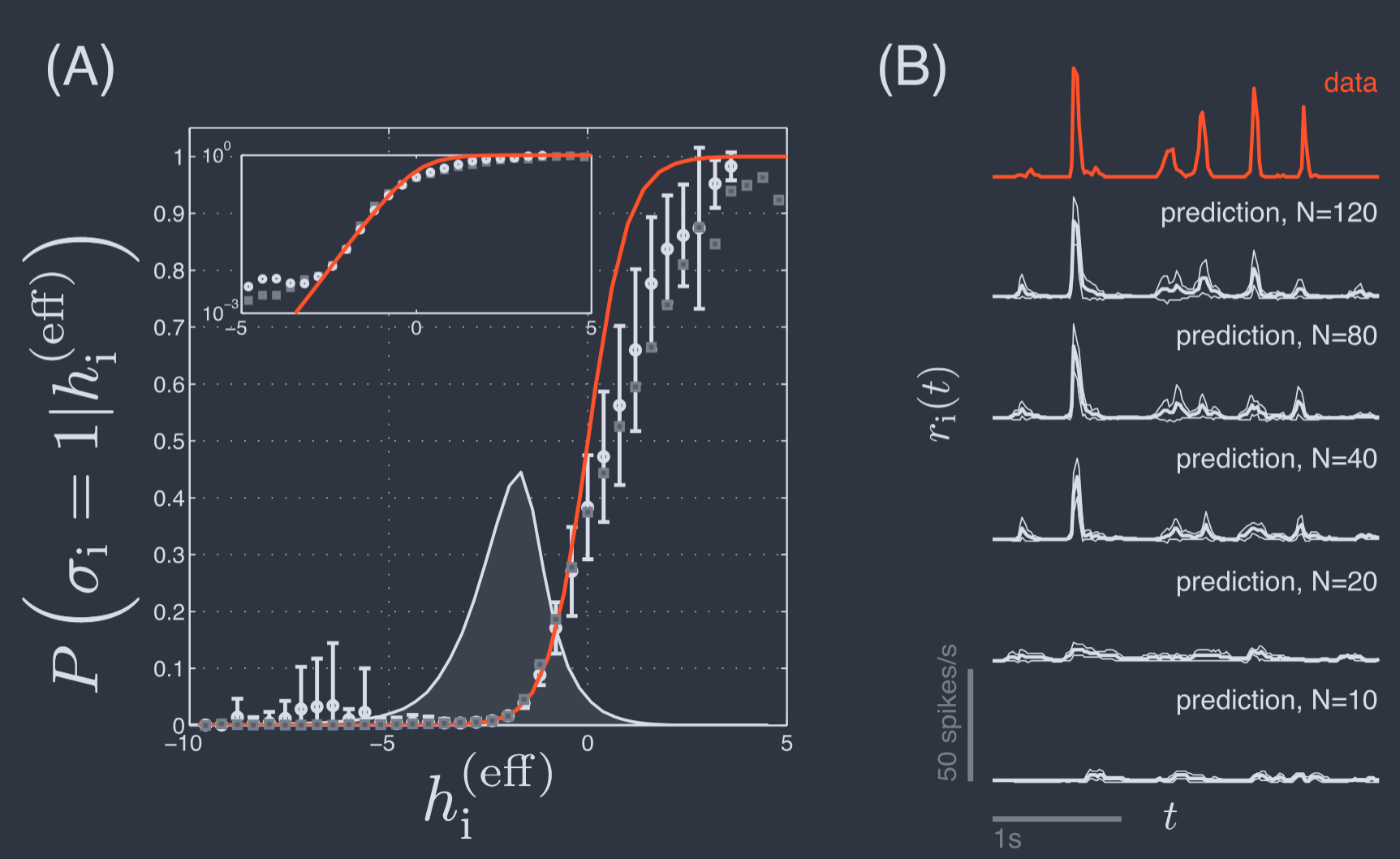
We see that the predictions of Eqs (B8) and (50) in the $K$–pairwise model agree well with experiment throughout the bulk of the distribution of effective fields, but that discrepancies arise in the tails. These deviations are $\sim 1.5\times$ the error bars of the measurement, but have some systematic structure, suggesting that we are capturing much but not quite all of the collective behavior under conditions where neurons are driven most strongly.

我们看到 $K$–成对模型中方程（B8）和（50）的预测与实验在有效场分布的主体部分很好地一致，但在尾部出现了偏差。这些偏差约为测量误差条的 $\sim 1.5\times$，但具有一些系统结构，表明我们正在捕捉大部分但并非全部的集体行为，在神经元受到最强驱动的条件下也是如此。

The results in Fig. 11A combine data across all times to estimate the probability of activity in one cell given the state of the rest of the network. It is interesting to unfold these results in time. In particular, the structure of the experiment was such that the retina saw the same movie many times, and so we can condition on a particular moment in the movie, as shown for one neuron in Fig 11B. It is conventional to plot not the probability of being active in a small bin but the corresponding “rate” (Rieke et al., 1997)

$$ r_{i}(t) = \langle\sigma_{i}(t)\rangle/\Delta\tau $$

where $\sigma_{i}(t)$ denotes the state of neuron $i$ at time $t$ relative to (in this case) the visual inputs. We see in the top trace of Fig. 11B that single neurons are active very rarely, with essentially zero probability of spiking between brief transients that generate on average one or a few spikes. This pattern is common in response to naturalistic stimuli, and very difficult to reproduce in models (Maheswaranathan et al., 2023).

翻译

图 11A 中的结果结合了所有时间的数据，以估计在给定网络其余部分状态时一个细胞的活动概率。有趣的是将这些结果展开在时间上。特别是，实验的结构是视网膜多次看到同一部电影，因此我们可以以电影中的特定时刻为条件，如图 11B 中所示的一个神经元。通常不绘制在小箱中活跃的概率，而是绘制相应的“速率”（Rieke 等人，1997）

$$ r_{i}(t) = \langle\sigma_{i}(t)\rangle/\Delta\tau $$

其中 $\sigma_{i}(t)$ 表示相对于（在这种情况下）视觉输入的时间 $t$ 神经元 $i$ 的状态。我们在图 11B 的顶部轨迹中看到，单个神经元非常罕见地活跃，在产生平均一个或几个尖峰的短暂瞬变之间几乎没有尖峰的概率。这种模式在对自然刺激的响应中很常见，并且在模型中很难再现（Maheswaranathan 等人，2023）。

The maximum entropy models provide an extreme opposite point of view, making no reference to the visual inputs; instead activity is determined by the state of the rest of the network. We see that this approach correctly predicts sparse activity, with near zero rate between transients that are timed correctly relative to the input. Although here we see just one cell, the average neuron exhibits an $r_{i}(t)$ that has $\sim 80%$ correlation with the theoretical predictions at $N = 120$. There is no sign of saturation, and it seems likely we would make even more precise predictions from models based on all $N\sim 200$ cells in this small patch of the retina. The possibility of predicting activity without reference to the visual input suggests that the “vocabulary” of the retina’s output is restricted, and that as with spelling rules this should allow for error-correction(Loback et al., 2017).

最大熵模型提供了一个极端相反的观点，不参考视觉输入；相反，活动由网络其余部分的状态决定。我们看到这种方法正确地预测了稀疏活动，在与输入相对正确定时的瞬变之间速率接近零。虽然这里我们只看到一个细胞，但平均神经元表现出与理论预测在 $N = 120$ 时约有 $\sim 80%$ 的相关性的 $r_{i}(t)$。没有饱和的迹象，并且似乎我们可以从基于视网膜这个小块中所有 $N\sim 200$ 个细胞的模型中做出更精确的预测。在不参考视觉输入的情况下预测活动的可能性表明，视网膜输出的“词汇”是受限的，并且就像拼写规则一样，这应该允许进行纠错（Loback 等人，2017）。

Perhaps the most basic prediction from maximum entropy models is the entropy itself. There are several ways that we can estimate the entropy. First, in the $K$-pairwise model we can see that the effective energy of the completely silent state, from Eq (46), is zero, which means that the probability of this state is just the inverse of the partition function. Further, in this model, the probability of complete silence matches what we observe experimentally. Thus we can estimate the free energy of the model from the data, and then we can estimate the mean energy of the model from Monte Carlo, giving us an estimate of the entropy. An alternative is to generalize the model by introducing a fictitious temperature, as will be discussed in §VI.B. Then at $T = 0$ the entropy must be zero and at $T\to\infty$ the entropy must be $N\log{2}$, while the derivative of the entropy is related as always to the heat capacity. Thus the entropy of our model for the real system at $T = 1$ becomes

$$ S_{N}(T=1) = \int_{0}^{1}\mathrm{d}T\frac{C_{v}(T)}{T} = N\log{2} - \int_{1}^{\infty}\mathrm{d}T\frac{C_{v}(T)}{T} $$

where the heat capacity is related as usual to the variance of the energy, $\begin{aligned}C_{v} = \frac{\langle (\delta E)^{2}\rangle}{T^{2}}\end{aligned}$, that we can estimate from Monte Carlo simulations at each $T$. There is also a check that the two estimates in Eq (52) should agree. All of these methods agree with one another at the percent level, with results shown in Fig. 12A.

也许最大熵模型的最基本预测是熵本身。我们可以通过几种方式来估计熵。首先，在 $K$-成对模型中，我们可以看到完全静止状态的有效能量，从方程（46）来看为零，这意味着该状态的概率只是配分函数的倒数。此外，在该模型中，完全静止的概率与我们在实验中观察到的相匹配。因此，我们可以从数据中估计模型的自由能，然后我们可以从蒙特卡罗中估计模型的平均能量，从而给出熵的估计。另一种方法是通过引入虚构温度来推广模型，如 §VI.B 中将讨论的那样。那么在 $T = 0$ 时熵必须为零，而在 $T\to\infty$ 时熵必须为 $N\log{2}$，而熵的导数一如既往地与热容有关。因此，我们对真实系统在 $T = 1$ 时模型的熵变为

$$ S_{N}(T=1) = \int_{0}^{1}\mathrm{d}T\frac{C_{v}(T)}{T} = N\log{2} - \int_{1}^{\infty}\mathrm{d}T\frac{C_{v}(T)}{T} $$

其中热容与能量的方差有关，$\begin{aligned}C_{v} = \frac{\langle (\delta E)^{2}\rangle}{T^{2}}\end{aligned}$，我们可以从每个 $T$ 的蒙特卡罗模拟中估计它。还有一个检查，即方程（52）中的两个估计应该是一致的。所有这些方法在百分比水平上彼此一致，结果如图 12A 所示。

FIG. 12 Entropy and coincidences in the activity of the retinal network (Tkaˇcik et al., 2014). (A) Entropy predicted in K–pairwise models (red) and in the approximation that all neurons are independent (grey). Models are constructed independently for many subgroups of size $N$ chosen out of the total population $N_{\text{max}} = 160$, and error bars include the variance across these groups. (B) Probability that two randomly chosen states of the network are the same, again for many subgroups of size $N$. Results for real data (black), shuffled data (grey), and the $K$–pairwise models (red).

图 12 视网膜网络活动中的熵和巧合（Tkaˇcik 等人，2014）。（A）K–成对模型中预测的熵（红色）和所有神经元独立的近似（灰色）。模型是从总人口 $N_{\text{max}} = 160$ 中选择的许多大小为 $N$ 的子组独立构建的，误差条包括这些组之间的方差。（B）随机选择的网络状态相同的概率，同样适用于许多大小为 $N$ 的子组。真实数据的结果（黑色）、洗牌数据（灰色）和 $K$–成对模型（红色）。

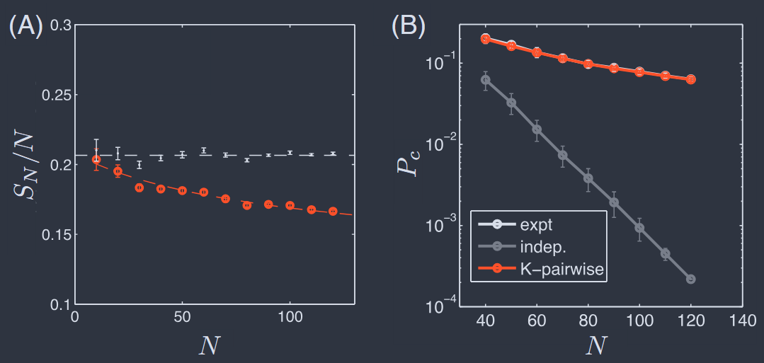
The $\sim 25%$ reduction in entropy is significant, but more dramatic (and testable) is the prediction that the distribution over states is extremely inhomogeneous. Recall that if the distribution is uniform over some effective number of states $\Omega_{\text{eff}}$ then the entropy is $S = \log{\Omega_{\text{eff}}}$ and the probability that two states chosen at random will be the same is $P_{c} = 1/\Omega_{\text{eff}}$ ; for non–uniform distributions we have $S\geq − \log(P_{c})$. If neurons were independent then with $N$ cells we would have $P_{c}\propto e^{−\alpha N}$, and this is what we see in the data once they are shuffled to remove correlations (Fig. 12B). But the real data show a much more gradual decay with $N$ , and this is captured perfectly by the $K$–pairwise maximum entropy models.

$\sim 25%$ 的熵减少是显著的，但更戏剧性（且可测试）的预测是状态分布极不均匀。回想一下，如果分布在某个有效状态数 Ωeff 上是均匀的，那么熵为 $S = \log{\Omega_{\text{eff}}}$，随机选择两个状态相同的概率为 $P_{c} = 1/\Omega_{\text{eff}}$；对于非均匀分布，我们有 $S\geq − \log(P_{c})$。如果神经元是独立的，那么对于 $N$ 个细胞，我们将有 $P_{c}\propto e^{−\alpha N}$，这正是我们在数据中看到的，一旦它们被洗牌以去除相关性（图 12B）。但真实数据随着 $N$ 显示出更渐进的衰减，而这正被 $K$–成对最大熵模型完美捕捉。

At $N = 120$ the logarithm of the coincidence probability (both measured and predicted) is an order of magnitude smaller than the entropy predicted by the model. Perhaps related is that the free energy per neuron—which, as discussed above, can be obtained directly from the probability of the fully silent state—also decreases dramatically as $N$ increases. At $N = 120$ the free energy is just a few percent of the either the entropy or the mean energy, reflecting near perfect cancelation between these terms; one can see this also in a much simpler model that only matches $P_{N}(K)$ and not the individual means or pairwise correlations (Tkacˇik et al., 2013). Importantly, these behaviors are captured by the K–pairwise model smoothly from $N < 40$ through $N > 100$, indicating that what we learned at more modest $N$ really does extrapolate up a scale comparable to the whole population of cells in a patch of the retina. We will have to work harder to decide if we can see the emergence of a true thermodynamic limit.

在 $N = 120$ 时，巧合概率的对数（测量和预测）比模型预测的熵小一个数量级。也许相关的是，每个神经元的自由能——正如上面讨论的那样，可以直接从完全静止状态的概率中获得——随着 $N$ 的增加也显著降低。在 $N = 120$ 时，自由能仅占熵或平均能量的百分之几，反映了这些项之间几乎完美的抵消；在一个只匹配 $P_{N}(K)$ 而不匹配单个均值或成对相关性的更简单模型中也可以看到这一点（Tkacˇik 等人，2013）。重要的是，这些行为通过 K–成对模型从 $N < 40$ 平滑地捕捉到 $N > 100$，表明我们在较适度的 $N$ 上学到的东西确实可以外推到与视网膜一块区域内细胞的整个群体相当的规模。我们将不得不更加努力地工作，以决定我们是否能够看到真正热力学极限的出现。

Finally, we should address the question of whether these results can be recovered as perturbations to a model of independent neurons. At lowest order in perturbation theory, there is a simple relationship between the observed correlations and the inferred interactions $J_{ij}$ in the pairwise model (Sessak and Monasson, 2009), and we can check this relationship against the values of $J_{ij}$ inferred from correctly matching the observed correlations. In the retina, large deviations from lowest order perturbation theory are visible already at $N = 15$, and correspondingly models built from the perturbative estimates of $J_{ij}$ are orders of magnitude further away from the data than the full model (Tkacˇik et al., 2014). Higher order perturbative contributions to the entropy would be comparable to one another for $N = 20$ retinal neurons even in a hypothetical network where all correlations were scaled down by a factor of two from the real data (Azhar and Bialek, 2010). We conclude that the success of maximum entropy models in describing networks of real neurons is not something we can understand in low order perturbation theory. Interestingly, simulations of models with pure 3– and 4-spin interactions at $N\sim 20$ show that pairwise maximum entropy models typically are good approximations to the real distribution both in the weak correlation limit and in the limit of strong, dense interactions (Merchan and Nemenman, 2016).

最后，我们应该解决这样一个问题：这些结果是否可以作为独立神经元模型的微扰来恢复。在微扰理论的最低阶中，观察到的相关性与成对模型中推断的相互作用 $J_{ij}$ 之间存在简单关系（Sessak 和 Monasson，2009），我们可以根据正确匹配观察到的相关性来检查这种关系与推断的 $J_{ij}$ 值之间的关系。在视网膜中，在 $N = 15$ 时已经可以看到与最低阶微扰理论的巨大偏差，因此从微扰估计的 $J_{ij}$ 构建的模型与完整模型相比，与数据相差几个数量级（Tkacˇik 等人，2014）。即使在一个假设网络中，所有相关性都比真实数据缩小了两倍，对于 $N = 20$ 个视网膜神经元，高阶微扰对熵的贡献也将彼此相当（Azhar 和 Bialek，2010）。我们得出结论，最大熵模型在描述真实神经元网络方面的成功不是我们可以在低阶微扰理论中理解的。有趣的是，在 $N\sim 20$ 时具有纯 3–和 4–自旋相互作用的模型模拟表明，成对最大熵模型通常是实际分布的良好近似，无论是在弱相关极限还是在强烈、密集相互作用的极限下（Merchan 和 Nemenman，2016）。

The retina is a very special part of the brain, and one might worry that the success of maximum entropy models is somehow tied to these special features. It thus is important that the same methods work in capturing the collective behavior of neurons in very distant parts of the brain. An example is in prefrontal cortex, which is involved in a wide range of higher cognitive functions.

视网膜是大脑中一个非常特殊的部分，人们可能会担心最大熵模型的成功与这些特殊特征有关。因此，同样的方法在捕捉大脑非常遥远部分神经元的集体行为方面也有效，这一点很重要。一个例子是在前额叶皮层，它参与了广泛的高级认知功能。

Experiments recording simultaneous activity from several tens of neurons in prefrontal cortex were analyzed with maximum entropy methods, and an example of the results is shown in Fig. 13 (Tavoni et al., 2017). We see that these models pass the same tests as in the retina, correctly predicting triplet correlations, the probability of $K$ out of $N$ cells being active simultaneously, and the probabilities for particular patterns of activity in subgroups of $N = 10$ cells. Extending this analysis across multiple experimental sessions it was possible to detect changes in the coupling matrix $J_{ij}$ as the animal learned to engage in different tasks. These changes were concentrated in subsets of cells which also were preferentially re–activated during sleep between sessions. One should be careful about giving too mechanistic an interpretation of the Ising models that emerge from these analyses, but it is exciting to see the structure of the models connect to independently measurable functional dynamics in the network. This is true even in the farthest reaches of the cortex, the regions of the brain that we use for thinking, planning, and deciding.

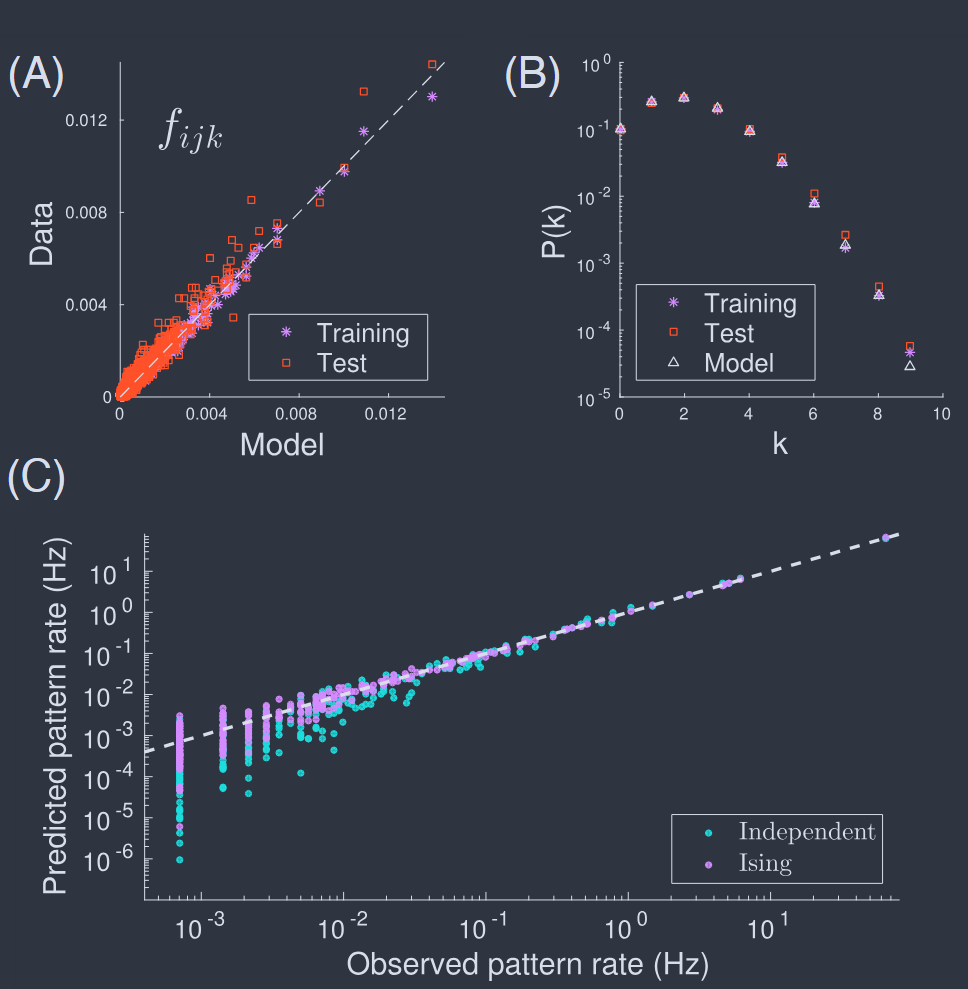
在前额叶皮层记录同时活动的几十个神经元的实验使用最大熵方法进行了分析，结果的一个例子如图 13 所示（Tavoni 等人，2017）。我们看到这些模型通过了与视网膜相同的测试，正确地预测了三元组相关性、$N$ 个细胞中有 $K$ 个同时活跃的概率，以及 $N = 10$ 个细胞子组中特定活动模式的概率。通过跨多个实验会话扩展此分析，可以检测到动物学习参与不同任务时耦合矩阵 $J_{ij}$ 的变化。这些变化集中在细胞子集中，这些细胞在会话之间的睡眠期间也被优先重新激活。我们应该小心不要对从这些分析中出现的伊辛模型给予过于机械的解释，但令人兴奋的是看到模型的结构与网络中独立可测量的功能动态相连接。即使在大脑皮层最远的区域，我们用于思考、计划和决策的大脑区域也是如此。

FIG. 13 Pairwise maximum entropy models describe collective behavior of $N = 37$ neurons in prefrontal cortex (Tavoni et al., 2017). (A) Observed vs predicted triplet correlations among all neurons. Training results (blue) are predictions from the same segment of the experiment where the pairwise correlations were measured; test results (red) are in a different segment of the experiment. (B) Probability that $K$ out of $N$ neurons are active simultaneously, comparing predictions of the model with data in training and test segments. (C) Rate at which patterns of spiking and silence appear in a subset of ten neurons, comparing predicted vs observed rates in an independent model (cyan) and in the pairwise model (blue).

图 13 成对最大熵模型描述前额叶皮层中 $N = 37$ 个神经元的集体行为（Tavoni 等人，2017）。（A）所有神经元之间观察到的与预测的三元组相关性。训练结果（蓝色）是从实验的同一段测量成对相关性的预测；测试结果（红色）在实验的不同部分。（B）$N$ 个神经元中有 $K$ 个同时活跃的概率，将模型的预测与训练和测试部分的数据进行比较。（C）在十个神经元子集中尖峰和静默模式出现的速率，在独立模型（青色）和成对模型（蓝色）中比较预测与观察到的速率。

The Ising model also gives us a way of exploring how the network would respond to hypothetical perturbations (Tavoni et al., 2016). If we increase the magnetic field uniformly across all the cells in the population of prefrontal neurons, the predicted changes in activity are far from uniform. For some cells the response and the derivative of the response (susceptibility) are on a scale expected if neurons respond independently to applied fields, but there are groups of cells that co–activate much more, with susceptibilities peaking at intermediate fields. It is tempting to think that these groups of cells have some functional significance, and this is supported by the fact that in the real data (with no fictitious fields) the groups of cells identified in this way remain co–activated over relatively long periods of time.

Ising 模型还为我们提供了一种探索网络如何响应假设扰动的方法（Tavoni 等人，2016）。如果我们在前额叶神经元群体中的所有细胞上均匀增加磁场，预测的活动变化远非均匀。对于某些细胞，响应及其响应的导数（易感性）处于预期的尺度上，如果神经元独立地响应施加的场，但有一些细胞群体共同激活得更多，在中间场处易感性达到峰值。令人想起的是，这些细胞群体具有某种功能意义，这得到了这样一个事实的支持：在真实数据中（没有虚构场），以这种方式识别的细胞群体在相对较长的时间内保持共同激活。

At the opposite extreme of organismal complexity, the worm C. elegans is an attractive target for these analyses because one can record not just from a large number of cells but from a large fraction of the entire brain at single cell resolution (§III.C). A major challenge is that these neurons do not generate discrete action potentials or bursts, so the signal are not naturally binary. A first step was to discretize the continuous fluorescence signals into three levels, and construct a Potts–like model that matched the population of each state and the probabilities that pairs of neurons are in the same state (Chen et al., 2019). Although these early data sets were limited, this simple model succeeded in predicting off–diagonal elements of the correlation matrix that were unconstrained, the probability that $K$ of $N$ neurons are in the same state, and the relative probabilities of different states in relation to the effective fields generated by the rest of the network. The fact that the same statistical physics approaches work in worms and in mammalian cortex is encouraging, though we should see more compelling tests with the next generation of experiments.

在有机体复杂性的相反极端，线虫 C. elegans 是这些分析的一个有吸引力的目标，因为人们不仅可以从大量细胞中记录，还可以从整个大脑的大部分区域以单细胞分辨率进行记录（§III.C）。一个主要的挑战是这些神经元不会产生离散的动作电位或爆发，因此信号不是自然二进制的。第一步是将连续的荧光信号离散化为三个水平，并构建一个 类 Potts 的模型，以匹配每个状态的人口以及成对神经元处于同一状态的概率（Chen 等人，2019）。尽管这些早期数据集有限，但这个简单的模型成功地预测了未受约束的相关矩阵的非对角元素，$N$ 个神经元中有 $K$ 个处于同一状态的概率，以及与网络其余部分产生的有效场相关的不同状态的相对概率。同样的统计物理方法在蠕虫和哺乳动物皮层中都有效，这令人鼓舞，尽管我们应该通过下一代实验看到更有说服力的测试。

A very different approach is to study networks of neurons that have been removed from the animal and kept alive in a dish. There is a long history of work on these “cultured networks,” and as noted above (§III.A) some of the earliest experiments recording from many neurons were done with networks that had been grown onto an array of electrodes (Pine and Gilbert, 1982). Considerable interest was generated by the observation that patterns of activity in cultured networks of cortical neurons consist of “avalanches” that exhibit at least some degree of scale invariance (§VI.A). Recent work returns to these data and shows that detailed patterns of spiking and silence are well described by pairwise maximum entropy models, reproducing triplet correlations and the probability that $K$ out of $N = 60$ neurons are active simultaneously (Sampaio Filho et al., 2024).

一种非常不同的方法是研究从动物体内移除并在培养皿中保持活力的神经元网络。这些“培养网络”有着悠久的研究历史，如上所述（§III.A），一些最早记录许多神经元的实验是使用生长在电极阵列上的网络进行的（Pine 和 Gilbert，1982）。人们对观察到皮层神经元培养网络中的活动模式由“雪崩”组成产生了相当大的兴趣，这些雪崩至少表现出某种程度的尺度不变性（§VI.A）。最近的工作回到了这些数据，并显示尖峰和静默的详细模式可以很好地用成对最大熵模型来描述，重现了三元组相关性以及 $N = 60$ 个神经元中有 $K$ 个同时活跃的概率（Sampaio Filho 等人，2024）。

As a final example we consider populations of $N\sim 100$ neurons in the mouse hippocampus (Meshulam et al., 2017). The hippocampus plays a central role in navigation and episodic memory, and is perhaps best known for its population of “place cells,” neurons that are active only when the animal moves to a particular position in its environment. First discovered in rodents (O’Keefe and Dostrovsky, 1971), it is thought that the whole population of these cells together provides the animal with a cognitive map (O’Keefe and Nadel, 1978). More recent work shows how this structure extends to three dimensions, and across hundreds of meters in bats (Tsoar et al., 2011; Yartsev and Ulanovsky, 2013).

作为最后一个例子，我们考虑小鼠海马体中 $N\sim 100$ 个神经元的群体（Meshulam 等人，2017）。海马体在导航和情节记忆中起着核心作用，或许最著名的是其“位置细胞”群体，这些神经元仅在动物移动到其环境中的特定位置时才活跃。最早在啮齿动物中发现（O’Keefe 和 Dostrovsky，1971），人们认为这些细胞的整个群体共同为动物提供了认知地图（O’Keefe 和 Nadel，1978）。最近的工作展示了这种结构如何扩展到三维，并跨越蝙蝠中的数百米（Tsoar 等人，2011；Yartsev 和 Ulanovsky，2013）。

As the animal explores its environment, or runs along a virtual track, the mean activity of individual neurons is quite small, as in the examples above. Most pairs of neuron have negative correlations, as expected if activity is tied to the position—if each cell is active in a different place, then on average one cell being active means that other cells must be silent, generating anti- correlations. Indeed it is tempting to make a model of the hippocampus in which some positional signal is computed by the brain, with inputs from many regions, and each cell in the hippocampus is active or silent depending on the value of this positional signal. This model is specified by the “place fields” of each cell, the probability that a cell is active as a function of position, and these can be estimated directly from the data; given the place fields all other properties of the network are determined with no adjustable parameters.

当动物探索其环境或沿着虚拟轨道运行时，单个神经元的平均活动相当小，如上面的例子所示。大多数神经元对具有负相关性，这符合预期，如果活动与位置相关——如果每个细胞在不同的位置活跃，那么平均而言，一个细胞活跃意味着其他细胞必须静默，从而产生反相关。实际上，构建一个海马体模型是很诱人的，在该模型中，大脑通过来自许多区域的输入计算某种位置信号，海马体中的每个细胞根据该位置信号的值处于活跃或静默状态。该模型由每个细胞的“位置场”指定，即细胞作为位置函数活跃的概率，这些可以直接从数据中估计；给定位置场，网络的所有其他属性都没有可调参数地确定。

The place field of cell $i$ is defined by the average activity conditional on the position $x$ along a track,

$$ \langle\sigma_{i}\rangle_{x} = F_{i}(x) $$

If activity in each cell depends independently on position, then the pairwise correlations are driven by the fact that all cells experience the same x, drawn from some distribution $P (x)$ across the experiment. The quantitative prediction is that

$$ \begin{aligned} C_{ij} &\equiv \langle\sigma_{i}\sigma_{j}\rangle - \langle\sigma_{i}\rangle\langle\sigma_{j}\rangle \\ &= \int\mathrm{d}x P(x)F_{i}(x)F_{j}(x) - \left[\int\mathrm{d}x P(x)F_{i}(x)\right]\left[\int\mathrm{d}x P(x)F_{j}(x)\right] \end{aligned} $$

The covariance matrix elements $C_{ij}$ have a pattern that is qualitatively similar to the real data, but quantitatively very far off. In particular the eigenvalue spectrum of the matrix predicted in this way falls very rapidly, while the real spectrum has a slow, nearly power–law decay (Meshulam et al., 2017). This is a first hint that the neurons in the hippocampal network share information, and hence exhibit collective behavior, beyond just place.

细胞 $i$ 的位置场由沿轨道位置 $x$ 条件下的平均活动定义，

$$ \langle\sigma_{i}\rangle_{x} = F_{i}(x) $$

如果每个细胞的活动独立地依赖于位置，那么成对相关性是由所有细胞经历相同的 x 驱动的，这些 x 是从实验中的某个分布 $P (x)$ 中抽取的。定量预测是

$$ \begin{aligned} C_{ij} &\equiv \langle\sigma_{i}\sigma_{j}\rangle - \langle\sigma_{i}\rangle\langle\sigma_{j}\rangle \\ &= \int\mathrm{d}x P(x)F_{i}(x)F_{j}(x) - \left[\int\mathrm{d}x P(x)F_{i}(x)\right]\left[\int\mathrm{d}x P(x)F_{j}(x)\right] \end{aligned} $$

协方差矩阵元素 $C_{ij}$ 具有与真实数据定性上相似的模式，但在定量上非常偏离。特别是，以这种方式预测的矩阵的特征值谱下降得非常快，而真实谱具有缓慢、近似幂律衰减（Meshulam 等人，2017）。这是一个初步的暗示，表明海马体网络中的神经元共享信息，因此表现出超越位置的集体行为。

A new generation of experiments monitoring 1000+ neurons in the hippocampus provides unique opportunities for theory, as discussed in §§V and VII below. Here we want to emphasize the way in which collective dynamics emerge from maximum entropy models of $N\sim 100$ cells. Equations (49, 50) and Figure 11 remind us that models for the joint distribution of activity in a neural population also predict the probability for one neuron to be active given the state of the rest of the network. We can go through the same exercise for a population of cells in the hippocampus: construct the pairwise maximum entropy model, and for each neuron at each moment compute the probability that it will be active given the state of all the other neurons; results are shown in Fig 14A.

新一代监测海马体中 1000 多个神经元的实验为理论提供了独特的机会，如下文 §§V 和 VII 所讨论的那样。在这里，我们想强调集体动力学如何从 $N\sim 100$ 个细胞的最大熵模型中出现。方程（49，50）和图 11 提醒我们，神经群体中活动联合分布的模型还预测了在网络其余部分状态给定的情况下一个神经元活跃的概率。我们可以对海马体中的细胞群体进行同样的练习：构建成对最大熵模型，并在每个时刻为每个神经元计算在所有其他神经元状态给定的情况下它将活跃的概率；结果如图 14A 所示。

Collective behavior in the mouse hippocampus (Meshulam et al., 2017). (A) Predicted probability of activity for single neurons, computed from the effective field in the pairwise maximum entropy model. Focus is on 32 place cells that should be active in sequence as the mouse runs along a virtual track. During the first run, cells 21–25 are predicted to “miss” their place fields, but all cells are predicted to be active in the second run. (B) Real data of place cell activity during two runs down the linear track, in the same time window as (A) and (C); note the missed events for cells 21–25 in the first run. (C) Predicted probability from the independent place cell model. There is no indication of when fields should be missed.

小鼠海马体中的集体行为（Meshulam 等人，2017）。（A）从成对最大熵模型中的有效场计算的单个神经元的预测活动概率。重点关注 32 个位置细胞，当小鼠沿着虚拟轨道运行时，这些细胞应该按顺序活跃。在第一次运行期间，预测细胞 21–25 会“错过”它们的位置场，但在第二次运行中预测所有细胞都会活跃。（B）与（A）和（C）相同时间窗口内线性轨道上两次运行期间位置细胞活动的真实数据；请注意第一次运行中细胞 21–25 的错过事件。（C）来自独立位置细胞模型的预测概率。没有迹象表明何时应该错过场。

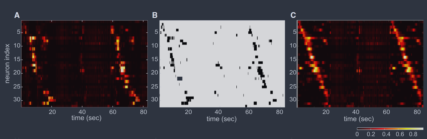
We see in Figure 14A that, roughly speaking, cells are predicted to be active in sequence. This makes sense since these are place cells, and the mouse is running at nearly constant speed along a virtual track, so cells with place fields arrayed along the track should be activated one after the other. Interestingly the calculation leading to this prediction makes no reference to the (virtual) position of the mouse, or even to the idea of place fields, but only to the dependence of activity in one cell on the rest of the network. In this window of time the mouse actually makes two trips along the track, and perhaps surprisingly the predictions for the two trips are different. On the first trip it is predicted that several of the cells will “miss” their place fields, while all cells should be active in sequence on the second trip. This is exactly what we see in the data (Fig 14B). If neurons were driven only by the animal’s position this wouldn’t happen (Fig 14C). Thus what might have seemed like unpredictable variation really reflects the collective behavior of the network, and is captured very well by the Ising model, with no additional parameters. We return to Ising models for the hippocampus in §V below.

我们在图 14A 中看到，大致来说，细胞被预测为按顺序活跃。这是有道理的，因为这些是位置细胞，小鼠以几乎恒定的速度沿着虚拟轨道运行，因此沿轨道排列的位置场的细胞应该一个接一个地被激活。有趣的是，导致这一预测的计算没有参考小鼠的（虚拟）位置，甚至没有参考位置场的概念，而只是参考一个细胞对网络其余部分活动的依赖。在这段时间内，小鼠实际上沿轨道进行了两次旅行，或许令人惊讶的是，两次旅行的预测是不同的。在第一次旅行中，预测有几个细胞会“错过”它们的位置场，而在第二次旅行中所有细胞都应该按顺序活跃。这正是我们在数据中看到的（图 14B）。如果神经元仅由动物的位置驱动，这种情况就不会发生（图 14C）。因此，看似不可预测的变化实际上反映了网络的集体行为，并且被 Ising 模型很好地捕捉到了，没有额外的参数。我们将在下面的 §V 中回到海马体的 Ising 模型。

Doing more and doing less

Is there any sense in which maximum entropy models are “better” than alternative models? The pairwise maximum entropy models are singled out because they have the minimal structure needed to match the mean activity and two–point correlations in the network. But how different are they from other models that would also match these data? We could imagine, for example, that once we specify the full matrix of correlations then the set of allowed models is very tightly clustered in its predictions about higher order structure in the patterns of activity, in which case saying that these models “work” doesn’t say much about the underlying physics.

最大熵模型在某种意义上是否比替代模型“更好”？成对最大熵模型之所以被单独挑选出来，是因为它们具有匹配网络中平均活动和两点相关性所需的最小结构。但是，它们与其他也能匹配这些数据的模型有多大不同呢？例如，我们可以想象，一旦我们指定了完整的相关矩阵，那么允许的模型集在其对活动模式中更高阶结构的预测中就会非常紧密地聚集，在这种情况下，说这些模型“有效”并不能说明潜在的物理学。

One can build a statistical mechanics on the space of probability distributions $p(\vec{\sigma})$, defining a “version space” by all the models that match a given set of pairwise correlations within some tolerance $\epsilon$. We can construct a Boltzmann weight over this space in which the entropy of the underlying distribution plays the role of the (negative) energy,

$$ Q[p(\vec{\sigma})]\propto \delta \left[1-\sum_{\vec{\sigma}}p(\vec{\sigma})\right]\mathbf{U}_{\epsilon}[p(\vec{\sigma};\{m_{i};C_{ij}\})]\times \exp\left[-\beta\sum_{\vec{\sigma}}p(\vec{\sigma})\ln{p(\vec{\sigma})}\right], $$

where the first term in the product enforces normalization, the second term selects distributions that match expectation values within $\epsilon$, and the last term is the Boltzmann weight (Obuchi et al., 2015). Note that this is the maximum entropy distribution of distributions (!) consistent with a particular mean value of the entropy and the measured expectation values. As $\beta\to\infty$, $Q$ condenses around the maximum entropy distribution, while as $\beta\to 0$ all distributions consistent with the expectation values are given equal weight.

我们可以在概率分布 $p(\vec{\sigma})$ 的空间上构建统计力学，通过在某个容差 $\epsilon$ 范围内匹配给定成对相关性的一组模型来定义“版本空间”。我们可以在这个空间中构建一个玻尔兹曼权重，其中基础分布的熵起着（负）能量的作用，

$$ Q[p(\vec{\sigma})]\propto \delta \left[1-\sum_{\vec{\sigma}}p(\vec{\sigma})\right]\mathbf{U}_{\epsilon}[p(\vec{\sigma};\{m_{i};C_{ij}\})]\times \exp\left[-\beta\sum_{\vec{\sigma}}p(\vec{\sigma})\ln{p(\vec{\sigma})}\right], $$

其中乘积中的第一项强制归一化，第二项选择在 $\epsilon$ 范围内匹配期望值的分布，最后一项是玻尔兹曼权重（Obuchi 等人，2015）。请注意，这是与熵的特定平均值和测量的期望值一致的分布的最大熵分布（！）。当 $\beta\to\infty$ 时，$Q$ 在最大熵分布周围凝结，而当 $\beta\to 0$ 时，与期望值一致的所有分布都被赋予相等的权重。

If the matrix $C_{ij}$ is chosen at random then one can use methods from the statistical mechanics of disordered systems to develop an analytic theory that compares the similarity of the true distribution to those drawn at random from the ensembles of distributions at varying $\beta$. In this random setting the maximum entropy models are not special, and in a rough sense all models that match the low–order correlations are equally good approximations (Obuchi et al., 2015). Importantly this is not true for the real data on retinal neurons, where the maximum entropy model gives a better description than the typical model that matches the pairwise correlations, and this advantage grows with $N$: “for large networks it is better to pick the most random model than to pick a model at random” (Ferrari et al., 2017).

如果随机选择矩阵 $C_{ij}$，那么可以使用无序系统统计力学的方法来开发一种分析理论，将真实分布与从不同 $\beta$ 的分布集合中随机抽取的分布进行比较。在这种随机设置中，最大熵模型并不特殊，从粗略意义上讲，所有匹配低阶相关性的模型都是同样好的近似（Obuchi 等人，2015）。重要的是，对于视网膜神经元的真实数据并非如此，其中最大熵模型比匹配成对相关性的典型模型提供了更好的描述，并且这种优势随着 $N$ 的增加而增长：“对于大型网络来说，选择最随机的模型比随机选择一个模型更好”（Ferrari 等人，2017）。

One way that we could do more in describing the patterns of neural activity is to address their time dependence more explicitly. In particular for the retina we know that the network is being driven by visual inputs. We can repeat the movie many times and ask about the mean activity of each cell at a given moment in the movie, $\langle\sigma_{i}(t)\rangle$. In addition, as before, we can measure the correlations between neurons at the same moment in time, $\langle\sigma_{i}(t)\sigma_{j}(t)\rangle$. Thus we want to find a model for the distribution over sequences or trajetcories of network states $P_{\text{traj}}[\vec{\sigma}(t)]$ that has maximal entropy and matches the time–dependent mean activity

$$ \begin{aligned} m_{i}(t) &\equiv \langle\sigma_{i}(t)\rangle_{\text{ext}}\\ &= \langle \sigma_{i}(t)\rangle_{P_{\text{traj}}} \end{aligned} $$

as well as the time averaged equal time correlations

$$ \begin{aligned} C_{ij} &\equiv \frac{1}{\widetilde{T}}\sum_{t}\langle\delta\sigma_{i}(t)\delta\sigma_{j}(t)\rangle_{\text{ext}}\\ &= \frac{1}{\widetilde{T}}\sum_{t}\langle\delta\sigma_{i}(t)\delta\sigma_{j}(t)\rangle_{P_{\text{traj}}} \end{aligned} $$

where $\widetilde{T}$ is the duration of our observations in units of the time bin width $\Delta\tau$.

我们可以通过更明确地解决它们的时间依赖性来更好地描述神经活动模式。特别是对于视网膜，我们知道网络正在被视觉输入驱动。我们可以多次重复电影，并询问电影中给定时刻每个细胞的平均活动，$\langle\sigma_{i}(t)\rangle$。此外，和以前一样，我们可以测量神经元在同一时间点的相关性，$\langle\sigma_{i}(t)\sigma_{j}(t)\rangle$。因此，我们想要找到一个关于网络状态序列或轨迹的分布模型 $P_{\text{traj}}[\vec{\sigma}(t)]$，该模型具有最大熵并匹配时间依赖的平均活动

$$ \begin{aligned} m_{i}(t) &\equiv \langle\sigma_{i}(t)\rangle_{\text{ext}}\\ &= \langle \sigma_{i}(t)\rangle_{P_{\text{traj}}} \end{aligned} $$

以及时间平均的等时相关性

$$ \begin{aligned} C_{ij} &\equiv \frac{1}{\widetilde{T}}\sum_{t}\langle\delta\sigma_{i}(t)\delta\sigma_{j}(t)\rangle_{\text{ext}}\\ &= \frac{1}{\widetilde{T}}\sum_{t}\langle\delta\sigma_{i}(t)\delta\sigma_{j}(t)\rangle_{P_{\text{traj}}} \end{aligned} $$

其中 $\widetilde{T}$ 是我们以时间箱宽度 $\Delta\tau$ 为单位的观察持续时间。

This is an instance of the general structure presented in §IV.A, where the first set of observables is of the form

$$ \{f_{\mu}\}\rightarrow\{f_{i,t}\} = \{\sigma_{i}(t)\} $$

To constrain the expectation value of each of these terms we need a separate Lagrange multiplier, and as before we think of these as local field that now depend on time, $\lambda_{i,t} = h_{i}(t)$. In addition we have observables of the form

$$ \{f_{\mu}\} \rightarrow \{f_{ij}\} = \left\{\sum_{t}\sigma_{i}(t)\sigma_{j}(t)\right\} $$

and for each of these we again have a separate Lagrange multiplier that we think of as a spin–spin coupling, $\lambda_{ij} = J_{ij}$. The general Eqs (20, 21) now take the form

$$ \begin{aligned} P_{\text{traj}}[\vec{\sigma}(t)] &= \frac{1}{Z_{\text{traj}}}\exp{(-E_{\text{traj}}[\vec{\sigma}(t)])}\\ E_{\text{traj}} &= \sum_{t}\sum_{i}h_{i}(t)\sigma_{i}(t) + \frac{1}{2}\sum_{t}\sum_{ij}J_{ij}\sigma_{i}(t)\sigma_{j}(t) \end{aligned} $$

In this class of models, correlations arise both because different neurons may be subject to correlated timedependent fields and because of effects intrinsic to the network. If all of the correlations were driven by visual inputs then matching the correlations would lead to $J_{ij} = 0$, but this never happens with real data.

这是 §IV.A 中介绍的一般结构的一个实例，其中第一组可观察量的形式为

$$ \{f_{\mu}\}\rightarrow\{f_{i,t}\} = \{\sigma_{i}(t)\} $$

为了约束这些项的期望值，我们需要一个单独的拉格朗日乘子，和以前一样，我们将这些视为现在依赖于时间的局部场，$\lambda_{i,t} = h_{i}(t)$。此外，我们还有以下形式的可观察量

$$ \{f_{\mu}\} \rightarrow \{f_{ij}\} = \left\{\sum_{t}\sigma_{i}(t)\sigma_{j}(t)\right\} $$

对于每个这些，我们再次有一个单独的拉格朗日乘子，我们将其视为自旋-自旋耦合，$\lambda_{ij} = J_{ij}$。一般方程（20，21）现在采用以下形式

$$ \begin{aligned} P_{\text{traj}}[\vec{\sigma}(t)] &= \frac{1}{Z_{\text{traj}}}\exp{(-E_{\text{traj}}[\vec{\sigma}(t)])}\\ E_{\text{traj}} &= \sum_{t}\sum_{i}h_{i}(t)\sigma_{i}(t) + \frac{1}{2}\sum_{t}\sum_{ij}J_{ij}\sigma_{i}(t)\sigma_{j}(t) \end{aligned} $$

在这类模型中，相关性既是因为不同的神经元可能受到相关的时间依赖场的影响，也是由于网络内在的影响。如果所有相关性都是由视觉输入驱动的，那么匹配相关性将导致 $J_{ij} = 0$，但在真实数据中这种情况从未发生过。