Today, neural network models are known to many different communities: physicists and applied mathematicians, computer scientists and engineers, neurobiologists and cognitive scientists. Neural networks are at the heart of an ongoing revolution in artificial intelligence, and are making their way into many aspects of scientific data analysis, from cell biology to CERN. Here we provide a brief (and perhaps idiosyncratic) reminder of how some of these ideas developed.

今天，神经网络模型为许多不同的群体所知：物理学家和应用数学家、计算机科学家和工程师、神经生物学家和认知科学家。神经网络是人工智能正在进行的革命的核心，并正在进入从细胞生物学到 CERN 的许多科学数据分析方面。在这里，我们简要（也许是特立独行地）回顾了一些这些想法是如何发展的。

Prehistoric times

The engagement of physicists with neurons and the brain has a long and fascinating history. Our modern understanding of electricity has its roots in the 1700s with observations on nerves and muscles. The understanding of optics and acoustics that emerged in the 1800s was continuous with the exploration of vision and hearing. This involved thinking not just about the optics of the eye or the mechanics of the inner ear, but about the inferences that our brains can derive from the data collected by these physical instruments.

物理学家与神经元和大脑的接触有着悠久而迷人的历史。我们对电的现代理解起源于 1700 年代对神经和肌肉的观察。19 世纪出现的光学和声学的理解与对视觉和听觉的探索是连续的。这不仅涉及眼睛的光学或内耳的力学，还涉及我们的大脑可以从这些物理仪器收集的数据中推断出的推论。

The idea that the brain is made out of discrete cells, connected by synapses, dates from late 1800s (Ram ́on y Cajal, 1894). The electrical signals from individual nerve cells (neurons) were first recorded in the 1920s, starting with the cells in sense organs that provide the input to the brain (Adrian, 1928). Observing these small signals required instruments no less sensitive than those in contemporary physics laboratories. The crucial observation is that neurons communicate by generating discrete, identical pulses of voltage across their membranes; these pulses are called action potentials or, more colloquially, spikes.

大脑由离散的细胞通过突触连接而成的想法可以追溯到 19 世纪末（Ram ́on y Cajal，1894 年）。个别神经细胞（神经元）的电信号最早在 1920 年代被记录下来，首先是提供大脑输入的感觉器官中的细胞（Adrian，1928 年）。观察这些微小信号需要与当代物理实验室中的仪器同样敏感。关键的观察是，神经元通过在其膜上产生离散的、相同的电压脉冲来进行通信；这些脉冲称为动作电位，或者更通俗地说，称为尖峰。

By the 1950s there was a clear mathematical description of the dynamics underlying the generation and propagation of spikes (Hodgkin and Huxley, 1952). Perhaps surprisingly, the terms in these equations could be taken literally as representing the action of real physical components—ion channel proteins that allow the flow of specific ions across the cell membrane, and which open and close (or “gate”) in response to the transmembrane voltage. The progress from macroscopic phenomenology to the dynamics of individual channels is a beautiful chapter in the interaction of physics and biology. The classic textbook account is Aidley (1998); Dayan and Abbott (2001) discuss phenomenological models for spiking activity; and a broader biological context is provided by Kandel et al. (2012). Rieke et al. (1997) describe the way in which sequences of spikes represent information about the sensory world, and Bialek (2012) connects channels and spikes to other problems in the physics of biological systems.

到了 1950 年代，人们已经对产生和传播尖峰的动力学有了清晰的数学描述（Hodgkin 和 Huxley，1952 年）。也许令人惊讶的是，这些方程中的术语可以被字面理解为代表真实物理组件的作用——允许特定离子穿过细胞膜流动的离子通道蛋白，这些蛋白会根据跨膜电压的变化而打开和关闭（或“门控”）。从宏观现象学到单个通道动力学的进展是物理学与生物学相互作用中的一个美丽篇章。经典的教科书是 Aidley（1998）；Dayan 和 Abbott（2001）讨论了尖峰活动的现象学模型；Kandel 等人（2012）提供了更广泛的生物学背景。Rieke 等人（1997）描述了尖峰序列如何表示有关感官世界的信息，Bialek（2012）将通道和尖峰与生物系统物理学中的其他问题联系起来。

Even before the mechanisms were clear, people began to think about how the quasi–digital character of spiking could be harnessed to do computations (McCulloch and Pitts, 1943). This work comes after the foundational work of Turing (1937) on universal computation, but before any practical modern computers. The goal of this work was to show that the basic facts known about neurons were sufficient to support computing essentially anything. On the one hand this is a very positive theoretical development: the brain could be a computer, in a deep sense. On the other hand it is disappointing, since if the brain is a universal computer there is not much more that one can say about the dynamics..

即使在机制尚不清楚之前，人们就开始思考如何利用尖峰的准数字特性来进行计算（McCulloch 和 Pitts，1943 年）。这项工作是在 Turing（1937 年）关于通用计算的基础性工作之后，但在任何实用的现代计算机之前。这项工作的目标是表明，已知的关于神经元的基本事实足以支持计算本质上的任何东西。一方面，这是一个非常积极的理论发展：大脑可以在深层意义上成为一台计算机。另一方面，这令人失望，因为如果大脑是一台通用计算机，那么关于动力学就没有太多可说的了。

The way in which computation emerges from neurons in this early work clearly involves interactions among large numbers of cells in a network. Although single neurons can have remarkably precise dynamics in relation to sensory inputs and motor outputs (Hires et al., 2015; Nemenman et al., 2008; Rieke et al., 1997; Srivastava et al., 2017), there are many indications that our perceptions and actions, thoughts and memories typically are connected to the activity in many hundreds, perhaps even hundreds of thousands of neurons. Relevant activity in these large networks must be coordinated or collective.

在这项早期工作中，计算是如何从神经元中涌现出来的，显然涉及网络中大量细胞之间的相互作用。尽管单个神经元在感官输入和运动输出方面可以具有非常精确的动力学（Hires 等人，2015 年；Nemenman 等人，2008 年；Rieke 等人，1997 年；Srivastava 等人，2017 年），但有许多迹象表明，我们的感知和行动、思想和记忆通常与数百甚至数十万个神经元的活动有关。这些大型网络中的相关活动必须是协调或集体的。

The idea that collective neural activity in the brain might be described with statistical mechanics was very much influenced by observations on the electroencephalogram or EEG (Wiener, 1958). The EEG is a macroscopic measure of activity, traditionally done simply by placing electrodes on the scalp, and the existence of the EEG is prima facie evidence that the electrical activity of many, many neurons must be correlated. There is also the remarkable story of a demonstration by Adrian, in which he sat quietly with his eyes closed with electrodes attached to his head. The signals, sent to an oscilloscope, showed the characteristic “alpha rhythm” that occurs in resting states, roughly an oscillation at ∼ 10 Hz. When asked to add two numbers in his head, the rhythm disappeared, replaced by less easily described patterns of activity (Adrian and Matthews, 1934). This should dispel any lingering doubts that your mental life is related to the electrical activity of your brain.

大脑中集体神经活动可能用统计力学来描述的想法，深受对脑电图或 EEG 观察的影响（Wiener，1958 年）。EEG 是一种宏观的活动测量，传统上只是通过在头皮上放置电极来完成，EEG 的存在是第一手证据，表明许多神经元的电活动必须是相关的。还有一个令人惊讶的故事，讲述了 Adrian 的一个演示，他安静地坐着，闭着眼睛，头上连接着电极。信号被发送到示波器上，显示出在静息状态下发生的特征性“α节律”，大约是 ∼ 10 Hz 的振荡。当被要求在脑海中加两个数字时，这种节律消失了，取而代之的是不那么容易描述的活动模式（Adrian 和 Matthews，1934 年）。这应该消除任何关于你对心智与大脑电活动相关的质疑。

In the simplest models for neural dynamics, we describe the state of each neuron i at time t by a binary or Ising variable $\sigma_{i}(t)$; $\sigma_{i}(t) = +1$ means that the neuron is active, and $\sigma_{i}(t) = 0$ means that the neuron is silent.2 We imagine the dynamics proceeding in discrete time steps $\Delta\tau$ . Each neuron sums inputs from other neurons, weighted by the strength $J_{ij}$ of the synapse or connection from cell $j\rightarrow i$, and neurons switch into the active state if the total input is above a threshold:

$$ \sigma_{i}(t+\Delta\tau) = \Theta\left[\sum_{j}J_{ij}\sigma_{j}(t)-\theta_{i}\right] $$

The nature of the dynamics is encoded in the matrix $J_{ij}$ of synaptic strengths. If we think about arbitrary matrices, then the dynamics can be arbitrarily complex; progress depends on simplifying assumptions. It is useful to organize our discussion around two extreme simplifications. But keep in mind as we follow these threads that many of the developments occurred in parallel, and that there was considerable crosstalk.

在神经动力学的最简单模型中，我们通过二进制或 Ising 变量 $\sigma_{i}(t)$ 来描述每个神经元 i 在时间 t 的状态；$\sigma_{i}(t) = +1$ 意味着神经元处于活跃状态，$\sigma_{i}(t) = 0$ 意味着神经元处于静默状态。我们想象动力学以离散时间步长 $\Delta\tau$ 进行。每个神经元对来自其他神经元的输入进行求和，这些输入由从细胞 $j\rightarrow i$ 的突触或连接的强度 $J_{ij}$ 加权，如果总输入超过阈值，神经元就会切换到活跃状态：

$$ \sigma_{i}(t+\Delta\tau) = \Theta\left[\sum_{j}J_{ij}\sigma_{j}(t)-\theta_{i}\right] $$

动力学的性质编码在突触强度矩阵 $J_{ij}$ 中。如果我们考虑任意矩阵，那么动力学可以是任意复杂的；进展取决于简化假设。围绕两个极端简化来组织我们的讨论是有用的。但请记住，在我们跟随这些线索时，许多发展是并行发生的，并且存在相当大的串扰。

From perceptrons to deep networks

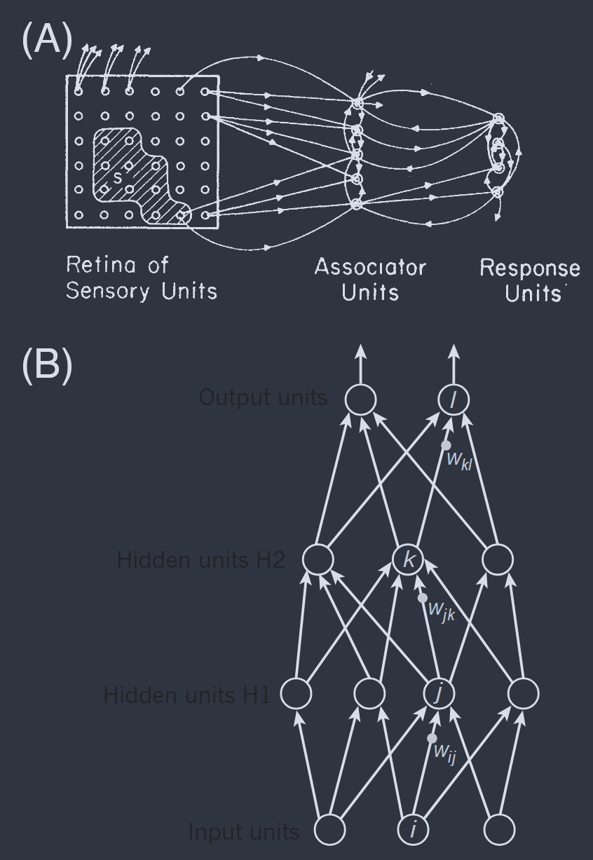
One popular simplification is to assume that $J_{ij}$ has a feed–forward, layered structure. This is the “perceptron” architecture (Block, 1962; Block et al., 1962; Rosenblatt, 1961), illustrated in Fig 1A, which is simpler to analyze precisely because there are no feedback loops. It is convenient to label the neurons also by the layer $l$ in which they reside, and to generalize from binary variables to continuous ones, so that

$$ x_{i}^{(l+1)} = g\left[\sum_{j}W_{ij}^{(l+1)}x_{j}^{(l)} - \theta_{i}^{(l+1)}\right] $$

where the propagation through layers replaces propagation through time and $g[\cdot]$ is a monotonic nonlinear function. Thus each neuron computes a single projection of its possible inputs from the previous layer, and then outputs a nonlinear function of this projection.

一种流行的简化是假设 $J_{ij}$ 具有前馈的分层结构。这是“感知器”架构（Block，1962 年；Block 等人，1962 年；Rosenblatt，1961 年），如图 1A 所示，正因为没有反馈回路，所以更容易分析。方便的是，还可以按它们所在的层 $l$ 来标记神经元，并将二进制变量推广为连续变量，因此

$$ x_{i}^{(l+1)} = g\left[\sum_{j}W_{ij}^{(l+1)}x_{j}^{(l)} - \theta_{i}^{(l+1)}\right] $$

其中通过层的传播取代了通过时间的传播，$g[\cdot]$ 是一个单调非线性函数。因此，每个神经元计算来自前一层的可能输入的单个投影，然后输出该投影的非线性函数。

In the limit that $g[\cdot]$ becomes a step function we recover binary variables and neuron $i$ in layer $l + 1$, can be thought of a dividing the space of its inputs in half, with a hyperplane perpendicular to the vector

$$ \vec{V} = \{V_{j}\} = \{W_{ij}^{(l+1)}\} $$

Thus the elementary computation is a binary classification of inputs,

$$ x\rightarrow y = \Theta(\vec{V}\cdot\vec{x}-\theta) $$

We could imagine having access to many examples of the input vector $\vec{x}$ labelled by the correct classification $y$, and thereby learning the optimal vector $\vec{V}$ . This picture of learning to classify was present already ∼1960, although it would take the full power of modern statistical physics to say that we really understand it. Crucially, if we think of the the $\{x_{i}\}$ or $\{\sigma_{i}\}$ as being the microscopic variables in the system and the $J_{ij}$ as being the interactions among these variables, then learning is statistical mechanics in the space of interactions (Gardner, 1988; Gardner and Derrida, 1988; Levin et al., 1990; Watkin et al., 1993).

在 $g[\cdot]$ 变成阶跃函数的极限下，我们恢复了二进制变量，层 $l + 1$ 中的神经元 $i$ 可以被认为是将其输入空间分成两半，具有垂直于向量的超平面

$$ \vec{V} = \{V_{j}\} = \{W_{ij}^{(l+1)}\} $$

因此，基本的计算是对输入的二元分类，

$$ x\rightarrow y = \Theta(\vec{V}\cdot\vec{x}-\theta) $$

我们可以想象获得许多输入向量 $\vec{x}$ 的示例，这些示例由正确的分类 $y$ 标记，从而学习最佳向量 $\vec{V}$。这种学习分类的图景已经出现在大约 1960 年，尽管需要现代统计物理学的全部力量才能说我们真正理解了它。关键是，如果我们将 $\{x_{i}\}$ 或 $\{\sigma_{i}\}$ 视为系统中的微观变量，而将 $J_{ij}$ 视为这些变量之间的相互作用，那么学习就是在相互作用空间中的统计力学（Gardner，1988 年；Gardner 和 Derrida，1988 年；Levin 等人，1990 年；Watkin 等人，1993 年）。

Although many of the computations done by the brain can be framed as classification problems, such as attaching names or words to images, very few can be solved by a single step of linear separation. Again this was clear at the start, but development of these ideas took decades. Enthusiasm was dampened by an emphasis on what two layer networks could not do (Minsky and Papert, 1969), but eventually it became clear that multilayer perceptrons are much more powerful (Lapedes and Farber, 1988; LeCun, 1987), and theorems were proven to show that these systems can approximate any function (Hornik et al., 1989). As with the simple perceptron, optimal weights $W$ can be learned by fitting to many examples of input/output pairs. Importantly this doesn’t require access to the “correct” answers at every layer; instead if we work with continuous variables then the goodness of fit across many layers can be differentiated using the chain rule, and errors propagated back through the network to adjust the weights (Rumelhart et al., 1986).

虽然大脑执行的许多计算都可以被框定为分类问题，例如将名称或单词附加到图像上，但很少有计算可以通过单一步骤的线性分离来解决。这一事实从一开始就很清楚，但这些想法的发展花费了几十年时间。由于强调两层网络无法完成的任务（Minsky 和 Papert，1969 年），热情有所减弱，但最终人们意识到多层感知器更加强大（Lapedes 和 Farber，1988 年；LeCun，1987 年），并且已经证明了这些系统可以近似任何函数的定理（Hornik 等人，1989 年）。与简单感知器一样，可以通过拟合许多输入/输出对的示例来学习最佳权重 $W$。重要的是，这不需要访问每一层的“正确”答案；相反，如果我们使用连续变量，那么通过链式法则可以区分多层之间的拟合优度，并将误差反向传播通过网络以调整权重（Rumelhart 等人，1986 年）。

Fast forward from the late 1980s to the mid 2010s. The few layers of early perceptrons became the many layers of “deep networks,” in the spirit of Fig 1B; comparing the two panels of Fig 1 emphasizes the continuity of ideas across the decades. Advances in computing power and storage made it possible not just to simulate these models efficiently, but to solve the problem of finding optimal synaptic weights by comparing against millions or even billions of examples. These explorations led to networks so large that the number of weights needed to specify the network vastly exceeded the number of examples. Contrary to well established intuitions these “over parameterized” models worked, generalizing to new examples rather than over–fitting to the training data. Although we don’t fully understand them, these developments have fueled a revolution in artificial intelligence (AI).

从 1980 年代后期快进到 2010 年代中期。早期感知器的几层变成了“深度网络”的多层，如图 1B 所示；比较图 1 的两个面板强调了几十年来思想的连续性。计算能力和存储的进步不仅使得高效地模拟这些模型成为可能，而且通过与数百万甚至数十亿个示例进行比较，解决了寻找最佳突触权重的问题。这些探索导致了如此庞大的网络，以至于指定网络所需的权重数量远远超过了示例的数量。与既定的直觉相反，这些“过参数化”模型有效，对新示例进行了泛化，而不是对训练数据进行了过拟合。尽管我们并不完全理解它们，但这些发展推动了人工智能（AI）的革命。

FIG. 1 Neural networks with a feed-forward architecture, or “perceptrons.” (A) An early version of the idea, from Block (1962). (B) A modern version, with additional hidden layers. The first steps in the modern AI revolution involved similar networks, with many hidden layers, that achieved human-level performance on image classification and other tasks (LeCun et al., 2015).

图一. 神经网络具有前馈架构，或“感知器”。（A）该想法的早期版本，来自 Block（1962 年）。（B）现代版本，具有额外的隐藏层。现代 AI 革命的第一步涉及类似的网络，具有许多隐藏层，在图像分类和其他任务上实现了人类水平的性能（LeCun 等人，2015 年）。

Symmetric networks

Feed–forward networks have the property that if $J_{ij}$ is nonzero, then $J_{ji} = 0$. Hopfield (1982, 1984) considered the opposite simplification: if neuron $i$ is connected to neuron $j$, then neuron $j$ is connected to neuron $i$, and the strength of the connection is the same, so that $J_{ij} = J_{ji}$. In this case the dynamics in Eq (1) have a Lyapunov function: at each time step the “energy”

$$ E = -\frac{1}{2}\sum_{ij}\sigma_{i}J_{ij}\sigma_{j} + \sum_{i}\theta_{i}\sigma_{i} $$

either decreases or stays constant. The evolution of the network state stops at local minima of the energy $E$, and only at these local minima. We recognize this energy function as an Ising model with pairwise interactions among the spins (neurons). This very explicit connection of neural dynamics to statistical physics triggered an avalanche of work, and textbook accounts of these ideas appeared quickly (Amit, 1989; Hertz et al., 1991).

前馈网络具有这样的属性：如果 $J_{ij}$ 非零，则 $J_{ji} = 0$。Hopfield（1982 年，1984 年）考虑了相反的简化：如果神经元 $i$ 与神经元 $j$ 相连，那么神经元 $j$ 也与神经元 $i$ 相连，并且连接的强度相同，因此 $J_{ij} = J_{ji}$。在这种情况下，方程（1）中的动力学具有 Lyapunov 函数：在每个时间步长中，“能量”

$$ E = -\frac{1}{2}\sum_{ij}\sigma_{i}J_{ij}\sigma_{j} + \sum_{i}\theta_{i}\sigma_{i} $$

要么减少，要么保持不变。网络状态的演变在能量 $E$ 的局部极小值处停止，并且仅在这些局部极小值处停止。我们将这个能量函数识别为具有自旋（神经元）之间成对相互作用的 Ising 模型。神经动力学与统计物理学的这种非常明确的联系引发了一系列工作，并且这些思想的教科书描述很快就出现了（Amit，1989 年；Hertz 等人，1991 年）。

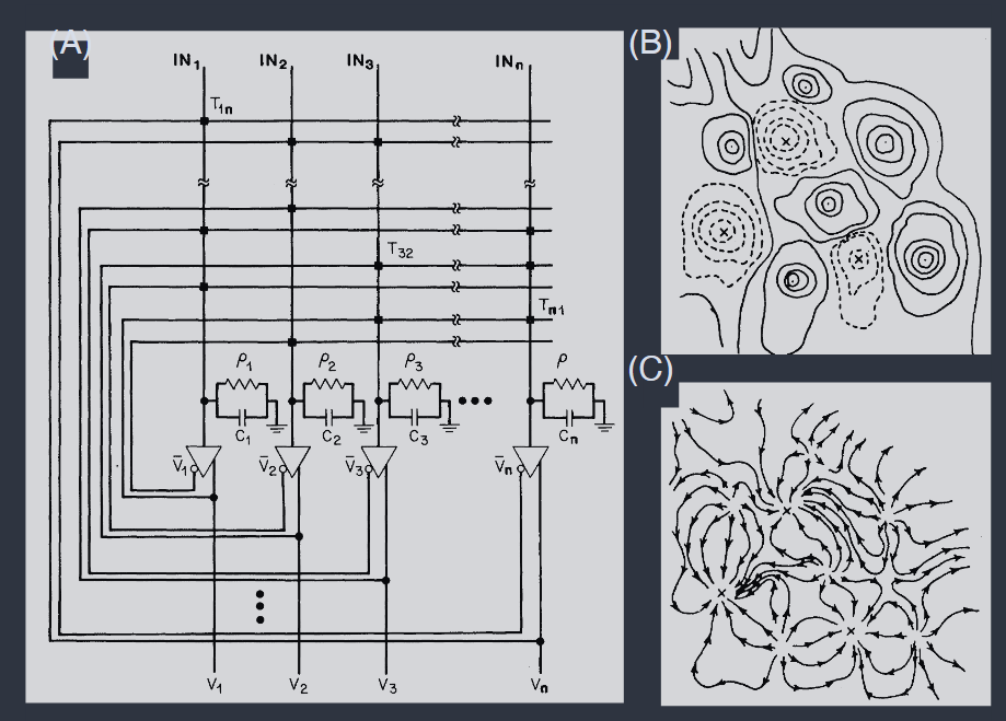
It was useful in visualizing the dynamics of symmetric networks that they can be realized by simple circuit components, using amplifiers with saturating outputs in place of neurons, as in Fig 2. As with perceptrons one generalize to soft spins, now in continuous time; one version of these dynamics is

$$ \tau\frac{\mathrm{d}x_{i}}{\mathrm{d}t} = -x_{i} + \sum_{j}J_{ij}g(x_{j}) $$

These models have the same collective behaviors as Ising spins (Hopfield, 1984).

在可视化对称网络的动力学时，它们可以通过简单的电路组件实现，这很有用，使用具有饱和输出的放大器代替神经元，如图 2 所示。与感知器一样，可以推广到软自旋，现在是在连续时间中；这些动力学的一个版本是

$$ \tau\frac{\mathrm{d}x_{i}}{\mathrm{d}t} = -x_{i} + \sum_{j}J_{ij}g(x_{j}) $$

这些模型具有与 Ising 自旋相同的集体行为（Hopfield，1984 年）。

FIG. 2 Equivalent circuit and dynamics in a symmetric network (Hopfield and Tank, 1986). (A) … (B) Schematic energy function for the circuit in (A); solid contours are above a mean level and dashed contours below, with X marking fixed points at the bottoms of energy valleys. (C) Corresponding dynamics, shown as a flow field. \

图二. 对称网络中的等效电路和动力学（Hopfield 和 Tank，1986 年）。（A）…（B）（A）中电路的示意能量函数；实线轮廓高于平均水平，虚线轮廓低于平均水平，X 标记能量谷底的固定点。（C）相应的动力学，显示为流场。

A crucial point is that one can “program” symmetric networks to place local minima at desired states. Since the dynamics will flow spontaneously toward these minima and stop, we can think of this programming as storing memories in the network, which then can be recovered by initializing the state anywhere in the relevant basin of attraction. Taking the mapping of the Lyapunov function to an energy more seriously, this memory storage represents a sculpting of the energy landscape, which is a more general idea. As an example, we can think about the evolution of amino acid sequences in proteins sculpting the energy landscape for folding.

一个关键点是，可以“编程”对称网络以在所需状态下放置局部极小值。由于动力学将自发地流向这些极小值并停止，我们可以将这种编程视为在网络中存储记忆，然后可以通过在相关吸引盆地中的任何位置初始化状态来恢复这些记忆。更认真地考虑 Lyapunov 函数到能量的映射，这种记忆存储代表了能量景观的雕刻，这是一个更一般的想法。作为一个例子，我们可以考虑蛋白质中氨基酸序列的演化，雕刻折叠的能量景观。

To illustrate the idea of memory storage, consider the case where the thresholds $\theta_{i} = 0$. Suppose we can construct a matrix of synaptic weights such that

$$ J_{ij} = J\xi_{i}\xi_{j} $$

where the $\xi_{i} = +1$ are again a set of (now fixed) binary or Ising variables. Then the energy function becomes

$$ E = -\frac{J}{2}\sum_{ij}\sigma_{i}\xi_{i}\xi_{j}\sigma_{j} = -\frac{J}2{}\left(\sum_{i}\sigma_{i}\xi_{i}\right)^{2} = -\frac{J}{2}\left(\vec{\sigma}\cdot\vec{\xi}\right)^{2} $$

Because both $\vec{\sigma}$ and $\vec{\xi}$ are binary vectors the energy is minimized when these vectors are equal. If want to be a bit fancier we can transform $\sigma_{i}\rightarrow \widetilde{\sigma}_{i} = \sigma_{i}\xi_{i}$, and we then realize that Eq (8) is gauge equivalent to the mean-field ferromagnet.

为了说明记忆存储的想法，考虑阈值 $\theta_{i} = 0$ 的情况。假设我们可以构建一个突触权重矩阵，使得

$$ J_{ij} = J\xi_{i}\xi_{j} $$

其中 $\xi_{i} = +1$ 再次是一组（现在固定的）二进制或 Ising 变量。那么能量函数变为

$$ E = -\frac{J}{2}\sum_{ij}\sigma_{i}\xi_{i}\xi_{j}\sigma_{j} = -\frac{J}2{}\left(\sum_{i}\sigma_{i}\xi_{i}\right)^{2} = -\frac{J}{2}\left(\vec{\sigma}\cdot\vec{\xi}\right)^{2} $$

由于 $\vec{\sigma}$ 和 $\vec{\xi}$ 都是二进制向量，当这些向量相等时能量最小化。如果想要更花哨一点，我们可以进行变换 $\sigma_{i}\rightarrow \widetilde{\sigma}_{i} = \sigma_{i}\xi_{i}$，然后我们意识到方程（8）在规范上等价于平均场铁磁体。

Crucially, we can generalize this construction,

$$ J_{ij} = J \left(\xi_{i}^{(1)}\xi_{j}^{(1)} + \xi_{i}^{(2)}\xi_{j}^{(2)} + \cdots + \xi_{i}^{(K)}\xi_{j}^{(K)}\right). $$

If network has $N$ neurons, and the number of these terms $K\ll N$ , then typically the vectors $\vec{\xi}^{(\mu)}$ are orthogonal, and the energy function will have multiple minima at $\vec{\sigma} = \vec{\xi}^{(\mu)}$: we have a model that stores $K$ memories.

关键是，我们可以推广这种构造，

$$ J_{ij} = J \left(\xi_{i}^{(1)}\xi_{j}^{(1)} + \xi_{i}^{(2)}\xi_{j}^{(2)} + \cdots + \xi_{i}^{(K)}\xi_{j}^{(K)}\right). $$

如果网络有 $N$ 个神经元，并且这些项的数量 $K\ll N$，那么通常向量 $\vec{\xi}^{(\mu)}$ 是正交的，并且能量函数将在 $\vec{\sigma} = \vec{\xi}^{(\mu)}$ 处具有多个极小值：我们有一个存储 $K$ 个记忆的模型。

To make this more rigorous let’s imagine that the states of the network are not just the minima of the energy function, but are drawn from a Boltzmann distribution at some inverse temperature $\beta$; it is plausible that this emerges from a noisy version of the dynamics in Eq (1). Then we have

$$ \begin{aligned} P(\vec{\sigma}) &= \frac{1}{Z}\exp{{-\beta E(\vec{\sigma})}} \\ E(\vec{\sigma}) &= -\frac{J_{0}}{N}\sum_{ij=1}^{N}\sum_{\mu=1}^{K}\sigma_{i}\xi_{i}^{\mu}\xi_{j}^{\mu}\sigma_{j} \end{aligned} $$

where we use the usual normalization of interactions by a factor $N$ to insure a thermodynamic limit. Because the stored patterns are fixed, this is a statistical mechanics problem with quenched disorder, a special kind of meanfield spin glass. As a first try we can take the stored patterns to be random vectors, which might make sense if we are describing a region of the brain where the mapping between the features of what we remember and the identities of neurons is very abstract. We can measure the success of recalling memories by measuring the order parameters

$$ m_{\mu} = \overline{\langle\vec{\xi}^{\mu}\cdot\vec{\sigma}\rangle} $$

where $\langle\cdots\rangle$ denotes an average over the “thermal” fluctuations in the neural state $\vec{\sigma}$ and $\overline{\cdots}$ denotes an average over the random choice of the patterns $\vec{\xi}^{\mu}$.

为了使这一点更加严格，让我们想象网络的状态不仅仅是能量函数的极小值，而是从某个逆温度 $\beta$ 的 Boltzmann 分布中抽取的；这可能是从方程（1）中的动力学的噪声版本中出现的。然后我们有

$$ \begin{aligned} P(\vec{\sigma}) &= \frac{1}{Z}\exp{{-\beta E(\vec{\sigma})}} \\ E(\vec{\sigma}) &= -\frac{J_{0}}{N}\sum_{ij=1}^{N}\sum_{\mu=1}^{K}\sigma_{i}\xi_{i}^{\mu}\xi_{j}^{\mu}\sigma_{j} \end{aligned} $$

其中我们使用通过因子 $N$ 的相互作用的通常归一化来确保热力学极限。由于存储的模式是固定的，这是一个具有淬火无序的统计力学问题，一种特殊类型的平均场自旋玻璃。作为第一次尝试，我们可以将存储的模式视为随机向量，如果我们正在描述大脑的一个区域，在那里我们记忆的特征与神经元的身份之间的映射非常抽象，这可能是有意义的。我们可以通过测量序参量来衡量回忆记忆的成功

$$ m_{\mu} = \overline{\langle\vec{\xi}^{\mu}\cdot\vec{\sigma}\rangle} $$

其中 $\langle\cdots\rangle$ 表示对神经状态 $\vec{\sigma}$ 中的“热”波动的平均，$\overline{\cdots}$ 表示对模式 $\vec{\xi}^{\mu}$ 的随机选择的平均。

Shortly before the introduction of these models, there had been dramatic developments in the statistical mechanics of disordered systems, including the solution of the fully mean–field Sherrington–Kirkpatrick spin glass model (Mezard et al., 1987). These tools could be applied to neural networks, resulting in a phase diagram mapping the order parameters $\{m_{\mu}\}$ as function of the fictitious temperature and the storage density $\alpha = K/N$ , all in the thermodynamic limit $N\to\infty$ (Amit et al., 1985, 1987). In the limit of zero temperature, below a critical $\alpha_{c} = 0.138$ only one of the $m_{\mu}$ will be nonzero, and it takes values close to one; this survives to finite temperatures. Thus there is a whole phase in which this model provides effective even if not quite perfect recall. By now we think of neural network models not as an application of statistical mechanics, but as a source of problems.

在引入这些模型之前，关于无序系统的统计力学已经有了戏剧性的进展，包括完全平均场 Sherrington–Kirkpatrick 自旋玻璃模型的解决方案（Mezard 等人，1987 年）。这些工具可以应用于神经网络，导致了一个相图，将序参量 $\{m_{\mu}\}$ 映射为虚拟温度和存储密度 $\alpha = K/N$ 的函数，所有这些都在热力学极限 $N\to\infty$ 中（Amit 等人，1985 年，1987 年）。在零温度的极限下，低于临界值 $\alpha_{c} = 0.138$ 时，只有一个 $m_{\mu}$ 将是非零的，并且它的值接近于一；这在有限温度下仍然存在。因此，在这个模型提供有效但不完全完美回忆的整个阶段中。到现在为止，我们认为神经网络模型不仅仅是统计力学的一个应用，而是问题的来源。

An important feature of the dynamics is that it is “associative.” Many initial states will relax to the same local minimum of the energy, which is equivalent to saying the same memory can be recalled from many different cues. In particular, we can imagine that the many bits represented by the state $\{\sigma_{i}\}$ can be grouped into features, e.g. parts of the image of a face, the sound of the person’s voice, $\dots$ . Under many conditions if one set of features is given and the others randomized, the nearest local minimum will have all the features correctly aligned (Hopfield, 1982). The fact that our mind conjures an image in response to a sound or a fragrance had once seemed mysterious, and this provides a path to demystification, built on the idea that stored and recalled memories are collective states of the network.

动力学的一个重要特征是它是“联想的”。许多初始状态将弛豫到能量的同一局部极小值，这相当于说同一记忆可以从许多不同的线索中回忆起来。特别是，我们可以想象由状态 $\{\sigma_{i}\}$ 表示的许多位可以分组为特征，例如面部图像的部分、该人的声音等。在许多条件下，如果给出一组特征并将其他特征随机化，则最近的局部极小值将使所有特征正确对齐（Hopfield，1982 年）。我们的心灵对声音或香味产生图像的事实曾经显得神秘，而这为去神秘化提供了一条途径，建立在存储和回忆的记忆是网络的集体状态的想法之上。

The synaptic matrix in Eq (9) has an important feature. Suppose that the network is currently in some state $\vec{\sigma}$ and we would like to add this state to the list of stored memories—i.e. we would like the network to learn the current state. Following Eq (9) we should change the synaptic weights

$$ J_{ij}\rightarrow J_{ij} + J\sigma_{i}\sigma_{j} $$

First we note that the connection between neurons $i$ and $j$ changes in a way that depends only on these two neurons. This locality of the learning rule is in a way remarkable, since we might have thought that sculpting the energy landscape would require more global manipulations. Second, the change in synaptic strength depends on the correlation between the pre–synaptic neuron $j$ and the post–synaptic neuron $i$: if the cells are active together, the synapse should be strengthened. This simple rule sometimes is summarized by saying that neurons that “fire together wire together,” and there is considerable evidence that real synapses change in this way. Indeed, although this idea has its origins in classical discussions (Hebb, 1949; James, 1904), more direct measurements demonstrating that correlated activity leads to long lasting increases of synaptic strength came only in the decade before Hopfield’s work (Bliss and Lømo, 1973).

方程（9）中的突触矩阵具有一个重要特征。假设网络当前处于某个状态 $\vec{\sigma}$，我们想将该状态添加到存储的记忆列表中——即我们希望网络学习当前状态。根据方程（9），我们应该改变突触权重

$$ J_{ij}\rightarrow J_{ij} + J\sigma_{i}\sigma_{j} $$

首先我们注意到，神经元 $i$ 和 $j$ 之间的连接以仅取决于这两个神经元的方式发生变化。这种学习规则的局部性在某种程度上是显著的，因为我们可能认为雕刻能量景观需要更全局的操作。其次，突触强度的变化取决于突触前神经元 $j$ 和突触后神经元 $i$ 之间的相关性：如果细胞一起活跃，突触应该被加强。这条简单的规则有时被总结为“共同发射的神经元共同连接”，并且有相当多的证据表明真实的突触以这种方式发生变化。事实上，尽管这个想法起源于经典讨论（Hebb，1949 年；James，1904 年），但在 Hopfield 的工作之前的十年中，才有更直接的测量表明相关活动会导致突触强度的长期增加（Bliss 和 Lømo，1973 年）。

In the first examples, the goal of computation was to recover a stored pattern from partial information (associative memory). Beyond memory, Hopfield and Tank (1985) soon showed that one could construct networks that solve classical optimization problems, and that many biologically relevant problems could be cast in this form (Hopfield and Tank, 1986). At the same time, the idea of simulated annealing (Kirkpatrick et al., 1983) led people to take much more seriously the mapping between “computational” problems of optimization and the “physical” problems of finding minimum energy states of many–body systems. This led, for example, to connections between statistical mechanics and computational complexity (Kirkpatrick and Selman, 1994; Monasson et al., 1999). From an engineering point of view, models for neural networks connected immediately to the possibility of using modern chip design methods to build analog, rather than digital circuits (Mead, 1989). Taken together, these simple symmetric models of neural networks formed a nexus among statistical physics, computer science, neurobiology, and engineering.

在最初的例子中，计算的目标是从部分信息中恢复存储的模式（联想记忆）。超越记忆，Hopfield 和 Tank（1985 年）很快表明，可以构建解决经典优化问题的网络，并且许多生物学相关的问题可以以这种形式进行投射（Hopfield 和 Tank，1986 年）。与此同时，模拟退火的想法（Kirkpatrick 等人，1983 年）使人们更加认真地对待“计算”优化问题与寻找多体系统最低能量状态的“物理”问题之间的映射。这导致了统计力学与计算复杂性之间的联系（Kirkpatrick 和 Selman，1994 年；Monasson 等人，1999 年）。从工程的角度来看，神经网络模型立即与使用现代芯片设计方法构建模拟而非数字电路的可能性相关联（Mead，1989 年）。总的来说，这些简单的对称神经网络模型形成了统计物理学、计算机科学、神经生物学和工程学之间的纽带。

Perspectives

Our emphasis in this review is on networks of real neurons. But it would be foolish to ignore what is happening in the world of engineered, artificial networks, which proceeds at a terrifying pace, realizing many of the old dreams for artificial intelligence (AI). Not so long ago we would have emphasized the tremendous progress being made on problems such as image recognition or game playing, where deep networks achieved something that approximates human level performance. Today, popular discussion is focused on generative AI, with networks that produces text and images that have a striking realism. Our theoretical understanding of why these things work remains quite weak. There are engineering questions about what practical problems can be solved with confidence by such systems, and ethical questions about how humanity will interact with these machines. The successes of AI even have led to some to suggest that the physicists’ notions of understanding might themselves be superseded. In opposition to this, many physicists are hopeful that ideas from statistical mechanics will help us build a better understanding of modern AI (Carleo et al., 2019; Mehta et al., 2019; Roberts and Yaida, 2022).

本文综述的重点是现实神经元网络。但忽视工程化的人工网络领域正在发生的事情是愚蠢的，这一领域以惊人的速度发展，实现了对人工智能（AI）的许多旧梦想。不久前，我们会强调在图像识别或游戏等问题上取得的巨大进展，在这些问题上，深度网络实现了接近人类水平的性能。今天，流行的讨论集中在生成式 AI 上，网络生成的文本和图像具有惊人的真实感。我们对这些事物为何有效的理论理解仍然相当薄弱。关于这些系统可以自信地解决哪些实际问题存在工程问题，以及关于人类将如何与这些机器互动的伦理问题。AI 的成功甚至导致一些人建议物理学家的理解概念本身可能会被取代。与此相反，许多物理学家希望统计力学的思想将帮助我们更好地理解现代 AI（Carleo 等人，2019 年；Mehta 等人，2019 年；Roberts 和 Yaida，2022 年）。

In a different direction, many physicists have been interested in more explicitly dynamical models of neural networks (Vogels et al., 2005), as in Eq (6). Guided by the statistical physics of disordered systems, one can study networks in which the matrix of synaptic connections is drawn at random, perhaps from an ensemble that captures some established features of real connectivity patterns. These same ideas can be used for probabilistic models of binary neurons; notable developments include the development of a dynamical mean–field theory for these systems (van Vreeswijk and Sompolinsky, 1998).

在另一个方向上，许多物理学家对神经网络的更明确的动态模型感兴趣（Vogels 等人，2005 年），如方程（6）所示。在无序系统的统计物理学的指导下，可以研究突触连接矩阵是随机抽取的网络，可能来自捕捉真实连接模式的一些已建立特征的集合。这些相同的思想可以用于二进制神经元的概率模型；值得注意的发展包括为这些系统开发动态平均场理论（van Vreeswijk 和 Sompolinsky，1998 年）。

Against the background of these theoretical developments, there has been a revolution in the experimental exploration of the brain, driven by techniques that combine methods from physics, chemistry and biology. We believe that this provides an unprecedented opportunity to connect statistical physics ideas to quantitative measurements on network dynamics in real brains. We turn first to an overview of the experimental state of the art.

在这些理论发展的背景下，大脑的实验探索发生了革命，这得益于结合了物理学、化学和生物学方法的技术。我们相信，这为将统计物理学思想与对真实大脑中网络动力学的定量测量联系起来提供了前所未有的机会。我们首先来概述一下实验的最新状态。