Introduction
The method by which brain produces mind has for centuries been discussed in terms of the most complex engineering and science metaphors of the day. Descartes described mind in terms of interacting vortices. Psychologists have metaphorized memory in terms of paths or traces worn in a landscape, a geological record of our experiences. To McCulloch and Pitts (1943) and von Neumann (1958), the appropriate metaphor was the digital computer, then in its infancy. The field of "neural networks" is the study of the computational properties and behavior of networks of "neuronlike" elements. It lies somewhere between a model of neurobiology and a metaphor for how the brain computes. It is inspired by two goals: to understand how neurobiology works, and to understand how to solve problems which neurobiology solves rapidly and effortlessly and which are very hard on present digital machines.
几个世纪以来,大脑产生心智的方法一直以当时最复杂的工程和科学隐喻来讨论。笛卡尔将心智描述为相互作用的漩涡。心理学家将记忆隐喻为景观中磨损的路径或痕迹,是我们经历的地质记录。对于 McCulloch 和 Pitts(1943)以及冯·诺依曼(1958)来说,适当的隐喻是当时还处于起步阶段的数字计算机。"神经网络" 领域是对 "类神经元" 元素网络的计算属性和行为的研究。它介于神经生物学模型和大脑如何计算的隐喻之间。它受两个目标的启发:理解神经生物学的工作原理,以及理解如何解决神经生物学能够快速轻松解决而当前数字机器却很难解决的问题。
Most physicists will find it obvious that understanding biology might help in engineering. The obverse engineering-toward-biological link can be made by testing a circuit of "model neurons" on a difficult real-world problem such as oral word recognition. If the "neural circuit" with some particular biological feature is capable of solving a real problem which circuits without that feature solve poorly, the plausibility that the biological feature selected is computationally useful in biology is bolstered. If not, then it is more plausible that the feature can be dispensed with in modeling biology. These are not strong arguments, but they do provide an approach to finding out what, of the myriad of details in neurobiology, is truly important and what is merely true. The study of a 1950 digital computer, in the spirit of neurobiology, would have a strong commitment to studying BaO, then the material of vacuum tube cathodes. The study of the digital computer in 1998 would have a strong commitment to SiO2, the essential insulating material below each gate. Yet the computing structure of the two machines could be identical, hidden amongst the lowest levels of detail. The study of "artificial neural networks" in the spirit of biology will relate to aspects of how neurobiology computes in the same sense that understanding the computer of 1998 relates to understanding the computer of 1950.
大多数物理学家会发现,理解生物学可能有助于工程学是显而易见的。可以通过在口语词识别等困难的现实问题上测试 "模型神经元" 电路来建立反向的工程朝向生物学的联系。如果具有某些特定生物特征的 "神经电路" 能够解决没有该特征的电路解决得很差的实际问题,那么所选择的生物特征在生物学中具有计算用途的可信度就会增强。反之,则更有可能在模拟生物学时可以省略该特征。这些不是强有力的论据,但它们确实提供了一种方法来找出神经生物学中无数细节中哪些是真正重要的,哪些只是正确的。以神经生物学的精神研究 1950 年的数字计算机,将强烈致力于研究 BaO(当时是真空管阴极的材料)。1998年对数字计算机的研究将强烈致力于 SiO2(每个门下方的基本绝缘材料)。然而,这两台机器的计算结构可能是相同的,隐藏在最低级别的细节中。以生物学精神研究 "人工神经网络" 将与理解 1998 年计算机与理解 1950 年计算机相关联,就像理解 1998 年计算机与理解 1950 年计算机一样。
BRAIN AS A COMPUTER
A digital machine can be programmed to compare a present image with a three-dimensional representation of a person, and thus the problem of recognizing a friend can be solved by a computation. Similarly, how to drive the actuators of a robot for a desired motion is a problem in classical mechanics that can be solved on a computer. While we may not know how to write efficient algorithms for these tasks, such examples do illustrate that what the nervous system does might be described as computation.
数字机器可以被编程为将当前图像与一个人的三维表示进行比较,因此识别朋友的问题可以通过计算来解决。类似地,如何驱动机器人的执行器以实现所需的运动是一个经典力学问题,可以在计算机上解决。虽然我们可能不知道如何为这些任务编写高效的算法,但这些例子确实说明了神经系统所做的事情可以描述为计算。
For present purposes, a computer can be viewed as an input-output device, with input and output signals that are in the same format (Hopfield, 1994). Thus in a very simple digital computer, the input is a string of bits (in time), and the output is another string of bits. A million axons carry electrochemical pulses from the eye to the brain. Similar signaling pulses are used to drive the muscles of the vocal tract. When we look at a person and say, "Hello, Jessica," our brain is producing a complicated transformation from one (parallel) input pulse sequence coming from the eye to another (parallel) output pulse sequence which results in sound waves being generated. The idea of composition is important in this definition. The output of one computer can be used as the input for another computer of the same general type, for they are compatible signals. Within this definition, a digital chip is a computer, and large computers are built as composites of smaller ones. Each neuron is a simple computer according to this definition, and the brain is a large composite computer.
对于目前的目的,计算机可以被视为一种输入输出设备,其输入和输出信号具有相同的格式(Hopfield,1994)。因此,在一个非常简单的数字计算机中,输入是一个比特串(随时间变化),输出是另一个比特串。一百万个轴突将来自眼睛的电化学脉冲传送到大脑。类似的信号脉冲用于驱动发声道的肌肉。当我们看着一个人并说 "你好,杰西卡" 时,我们的大脑正在将来自眼睛的一个(并行)输入脉冲序列转换为另一个(并行)输出脉冲序列,从而产生声波。组合的概念在这个定义中很重要。一个计算机的输出可以用作另一个相同类型计算机的输入,因为它们是兼容的信号。在这个定义中,数字芯片是一个计算机,而大型计算机是由较小的计算机组成的复合体。根据这个定义,每个神经元都是一个简单的计算机,而大脑则是一个大型复合计算机。
COMPUTERS AS DYNAMICAL SYSTEMS
The operation of a digital machine is most simply illustrated for batch-mode computation. The computer has $N$ storage registers, each storing a single binary bit. The logical state of the machine at a particular time is specified by a vector $10010110000\cdots$ of $N$ bits. The state changes each clock cycle. The transition map, describing which state follows which, is implicitly built into the machine by its design. The computer can thus be described as a dynamical system that changes its discrete state in discrete time, and the computation is carried out by following a path in state space.
数字机器的操作最简单地通过批处理计算来说明。计算机有 $N$ 个存储寄存器,每个寄存器存储一个二进制位。机器在特定时间的逻辑状态由一个 $N$ 位的向量 $10010110000\cdots$ 指定。状态在每个时钟周期都会改变。描述哪个状态跟随哪个状态的转换映射是通过其设计隐式构建到机器中的。因此,计算机可以被描述为一个在离散时间内改变其离散状态的动态系统,计算是通过在状态空间中跟随一条路径来完成的。
The user of the machine has no control over the dynamics, which is determined by the state transition map. The user’s program, data, and a standard initialization procedure prescribe the starting state of the machine. In a batch-mode computation, the answer is found when a stable point of the discrete dynamical system is reached, a state from which there are no transitions. A particular subset of the state bits (e.g., the contents of a particular machine register) will then describe the desired answer.
机器的用户无法控制动态,动态由状态转换映射决定。用户的程序、数据和标准初始化过程规定了机器的起始状态。在批处理计算中,当达到离散动态系统的稳定点时,就会找到答案,即没有转换的状态。然后,状态位的特定子集(例如,特定机器寄存器的内容)将描述所需的答案。
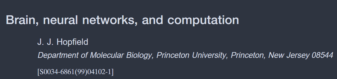
Batch-mode analog computation can be similarly described by using continuous variables and continuous time. The idea of computation as a process carried out by a dynamical system in moving from an initial state to a final state is the same in both cases. In the analog case, the possible motions in state space describe a flow field as in Fig. 1, and computation done by moving with this flow from start to end. (Real "digital" machines contain only analog components; the digital description is a representation in fewer variables which contains the essence of the continuous dynamics.)
批处理模拟计算也可以通过使用连续变量和连续时间来类似地描述。作为动态系统通过从初始状态移动到最终状态来完成的过程的计算概念在两种情况下都是相同的。在模拟情况下,状态空间中的可能运动描述了图 1 中的流场,计算是通过随该流动从开始到结束来完成的。(真正的 "数字" 机器只包含模拟组件;数字描述是在更少变量中的一种表示,包含了连续动态的本质。)
The flow field of a simple analog computer. The stable points of the flow, marked by $x$'s, are possible answers. To initiate the computation, the initial location in state space must be given. A complex analog computer would have such a flow field in a very large number of dimensions.
简单模拟计算机的流场。流的稳定点由 $x$ 标记,是可能的答案。要启动计算,必须给出状态空间中的初始位置。复杂的模拟计算机会具备一个这样的极高维数的流场。
DYNAMICAL MODEL OF NEURAL ACTIVITY
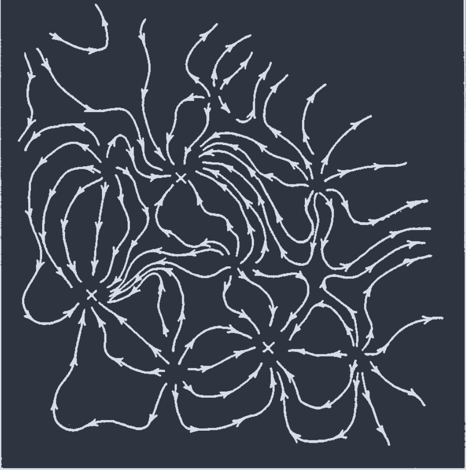
The anatomy of a "typical" neuron in a mammalian brain is sketched in Fig. 2 (Kandel, Schwartz, and Jessell, 1991). It has three major regions: dendrites, a cell body, and an axon. Each cell is connected by structures called synapses with approximately 1000 other cells. Inputs to a cell are made at synapses on its dendrites. The output of that cell is through synapses made by its axon onto the dendrites of other cells. The interior of the neuron is surrounded by a membrane of high resistivity and is filled with a conducting ionic solution. Ion-specific pumps transport ions across the membrane, maintaining an electrical potential difference between the inside and the outside of the cell. Ion-specific channels whose electrical conductivity is voltage dependent and dynamic play a key role in the evolution of the "state" of a neuron.
哺乳动物大脑中 "典型" 神经元的解剖结构如图 2 所示(Kandel、Schwartz 和 Jessell,1991)。它有三个主要区域:树突、细胞体和轴突。每个细胞通过称为突触的结构与大约 1000 个其他细胞连接。对细胞的输入是在其树突上的突触处进行的。该细胞的输出是通过其轴突在其他细胞的树突上形成的突触。神经元的内部被高电阻率的膜包围,并充满了导电离子溶液。离子特异性泵将离子运输穿过膜,维持细胞内外之间的电位差。电导率依赖于电压且动态变化的离子特异性通道在神经元 "状态" 的演变中起着关键作用。
A sketch of a neuron and its style of interconnections. Axons may be as long as many centimeters, though most are on the scale of a millimeter. Typical cell bodies are a few microns in diameter.
神经元及其互连方式的示意图。轴突可能长达数厘米,尽管大多数轴突的长度在毫米级别。典型的细胞体直径为几微米。
A simple "integrate and fire" model captures much of the mathematics of what a compact nerve cell does (Junge, 1981). Figure 3 shows the time-dependent voltage difference between the inside and the outside of a simple functioning neuron. The electrical potential is generally slowly changing, but occasionally there is a stereotype voltage spike of about two milliseconds duration. Such a spike is produced every time the interior potential of this cell rises above a threshold, $u_{\text{thresh}}$, of about 53 millivolts. The voltage then resets to a $u_{\text{reset}}$ of about 270 millivolts. This "action potential" spike is caused by the dynamics of voltage-dependent ionic conductivities in the cell membrane. If an electrical current is injected into the cell, then except for the action potentials, the interior potential approximately obeys
$$ C\frac{\mathrm{d}u}{\mathrm{d}t} = -\frac{u-u_{\text{rest}}}{R} + i(t) $$
where $R$ is the resistance of the cell membrane, $C$ the capacitance of the cell membrane, and $u_{\text{rest}}$ is the potential to which the cell tends to drift. If $i(t)$ is a constant $i_{c}$ , then the cell potential will change in an almost linear fashion between $u_{\text{rest}}$ and $u_{\text{thresh}}$ . An action potential will be generated each time $u_{\text{thresh}}$ is reached, resetting $u$ to $u_{\text{reset}}$ similar to what is seen in Fig. 3. The time $P$ between the equally spaced action potentials when $R$ is very large is
$$ P = C\frac{u_{\text{thresh}} - u_{\text{rest}}}{i_{c}},\quad \text{or firing rate}\quad \frac{1}{P}\sim i_{c} $$
If $i_{c}$ is negative, no action potentials will be produced. The firing rate $1/P$ of a more realistic cell is not simply linear in $i_{c}$, but asymptotes to a maximum value of about 500 per second (due to the finite time duration of action potentials). It may also have a nonzero threshold current due to leakage currents (of either sign) in the membrane.
一个简单的 "积分和发射" 模型捕捉了紧凑神经细胞所做的许多数学内容(Junge,1981)。图 3 显示了简单功能神经元内外之间的时变电压差。电位通常缓慢变化,但偶尔会出现大约两毫秒持续时间的典型电压峰值。每当该细胞的内部电位上升到大约 53 毫伏的阈值 $u_{\text{thresh}}$ 以上时,就会产生这样的峰值。然后,电压重置为大约 270 毫伏的 $u_{\text{reset}}$。这种 "动作电位" 峰值是由细胞膜中电压依赖性离子电导的动态引起的。如果向细胞注入电流,那么除了动作电位外,细胞内部电位大致遵循
$$ C\frac{\mathrm{d}u}{\mathrm{d}t} = -\frac{u-u_{\text{rest}}}{R} + i(t) $$
其中 $R$ 是细胞膜的电阻,$C$ 是细胞膜的电容,$u_{\text{rest}}$ 是细胞倾向于漂移到的电位。如果 $i(t)$ 是一个常数 $i_{c}$,那么细胞电位将在 $u_{\text{rest}}$ 和 $u_{\text{thresh}}$ 之间以几乎线性的方式变化。每次达到 $u_{\text{thresh}}$ 时都会产生一个动作电位,将 $u$ 重置为类似于图 3 中所示的 $u_{\text{reset}}$。当 $R$ 非常大时,等间隔动作电位之间的时间 $P$ 为
$$ P = C\frac{u_{\text{thresh}} - u_{\text{rest}}}{i_{c}},\quad \text{or firing rate}\quad \frac{1}{P}\sim i_{c} $$
如果 $i_{c}$ 为负,则不会产生动作电位。更现实的细胞的发射率 $1/P$ 并不是简单地与 $i_{c}$ 成线性关系,而是渐近于每秒约 500 的最大值(由于动作电位的有限时间持续)。它也可能由于膜中的泄漏电流(无论符号如何)而具有非零阈值电流。
Action potentials will be taken to be $\delta$ functions, lasting a negligible time. They propagate at constant velocity along axons. When an action potential arrives at a synaptic terminal, it releases a neurotransmitter which activates specific ionic conductivity channels in the postsynaptic dendrite to which it makes contact (Kandel, Schwartz, and Jessell, 1991). This short conductivity pulse can be modeled by
$$ \begin{aligned} \sigma(t) &= 0\quad &t<t_{0}\\ &= s_{kj}\exp{[-(t-t_{0})/\tau]}\quad &t>t_{0} \end{aligned} $$
The maximum conductivity of the postsynaptic membrane in response to the action potential is $s$. The ionspecific current which flows is equal to the chemical potential difference $V_{\text{ion}}$ times $s(t)$. Thus at a synapse from cell $j$ to cell $k$, an action potential arriving on axon $j$ at time $t_{0}$ results in a current
$$ \begin{aligned} i_{kj}(t) &= 0\quad &t<t_{0}\\ &= S_{kj}\exp{[-(t-t_{0})/\tau]}\quad &t>t_{0} \end{aligned} $$
flows into the cell $k$. The parameter $S_{kj} = V_{\text{ion}}s_{kj}$ can take either sign. Define the instantaneous firing rate of neuron $k$, which generates action potentials at times $t_{n}^{k}$, as
$$ f_{k}(t) = \sum_{n}\delta(t-t_{n}^{k}) $$
By differentiation and substitution
$$ \frac{\mathrm{d}i_{k}}{\mathrm{d}t} = -\frac{i_{k}}{\tau} + \sum_{j}S_{kj} \cdot f_{j}(t) + \text{another term if a sensory cell} $$
This equation, though exact, is awkward to deal with because the times at which the action potentials occur are only implicitly given.
动作电位将被视为持续时间可忽略的 $\delta$ 函数。它们以恒定速度沿轴突传播。当动作电位到达突触末端时,它会释放一种神经递质,激活与其接触的突触后树突中的特定离子电导通道(Kandel、Schwartz 和 Jessell,1991)。这种短暂的电导脉冲可以通过以下方式建模
$$ \begin{aligned} \sigma(t) &= 0\quad &t<t_{0}\\ &= s_{kj}\exp{[-(t-t_{0})/\tau]}\quad &t>t_{0} \end{aligned} $$
突触后膜对动作电位的最大电导为 $s$。流动的离子特异性电流等于化学势差 $V_{\text{ion}}$ 乘以 $s(t)$。因此,在从细胞 $j$ 到细胞 $k$ 的突触处,在时间 $t_{0}$ 在轴突 $j$ 上到达的动作电位会导致一个电流
$$ \begin{aligned} i_{kj}(t) &= 0\quad &t<t_{0}\\ &= S_{kj}\exp{[-(t-t_{0})/\tau]}\quad &t>t_{0} \end{aligned} $$
流入细胞 $k$。参数 $S_{kj} = V_{\text{ion}}s_{kj}$ 可以取任意符号。定义神经元 $k$ 的瞬时发射率,该神经元在时间 $t_{n}^{k}$ 产生动作电位,为
$$ f_{k}(t) = \sum_{n}\delta(t-t_{n}^{k}) $$
通过微分和替换
$$ \frac{\mathrm{d}i_{k}}{\mathrm{d}t} = -\frac{i_{k}}{\tau} + \sum_{j}S_{kj} \cdot f_{j}(t) + \text{another term if a sensory cell} $$
这个方程虽然是精确的,但处理起来很尴尬,因为动作电位发生的时间只是隐式给出的。
The usual approximation relies on there being many contributions to the sum in Eq. (6) during a reasonable time interval due to the high connectivity. It should then be permissible to ignore the spiky nature of $f_{j}(t)$, replacing it by a convolution with a smoothing function. In addition, the functional form of $V(i_{c})$ is presumed to hold when $i_{c}$ is slowly varying in time. What results is like Eq. (6), but with fj(t) now a smooth function given by $f_{j}(t) = V[i_{j}(t)] = V[i_{j}(t)]$:
$$ \frac{\mathrm{d}i_{k}}{\mathrm{d}t} = -\frac{i_{k}}{\tau} + \sum_{j}S_{kj} \cdot V[i_{j}(t)] + I_{k}(\text{last term only if a sensory cell}) $$
The main effect of the approximation, which assumes no strong correlations between spikes of different neurons, is to neglect shot noise. (Electrical circuits using continuous variables are based on a similar approximation.) While equations of this structure are in common use, they have somewhat evolved, and do not have a sharp original reference.
通常的近似依赖于由于高连接性,在合理的时间间隔内对方程(6)中的总和有许多贡献。然后应该允许忽略 $f_{j}(t)$ 的尖峰性质,用与平滑函数的卷积来替代它。此外,当 $i_{c}$ 随时间缓慢变化时,假定 $V(i_{c})$ 的函数形式成立。结果类似于方程(6),但现在 fj(t) 是由 $f_{j}(t) = V[i_{j}(t)] = V[i_{j}(t)]$ 给出的平滑函数:
$$ \frac{\mathrm{d}i_{k}}{\mathrm{d}t} = -\frac{i_{k}}{\tau} + \sum_{j}S_{kj} \cdot V[i_{j}(t)] + I_{k}(\text{last term only if a sensory cell}) $$
该近似的主要效果是假设不同神经元的峰值之间没有强相关性,从而忽略了散弹噪声。(使用连续变量的电路基于类似的近似。)虽然这种结构的方程被广泛使用,但它们已经有所发展,并且没有明确的原始参考文献。
THE DYNAMICS OF SYNAPSES
The second dynamical equation for neuronal dynamics describes the changes in the synaptic connections. In neurobiology, a synapse can modify its strength or its temporary behavior in the following ways:
- As a result of the activity of its presynaptic neuron, independent of the activity of the postsynaptic neuron.
- As a result of the activity of its postsynaptic neuron, independent of the activity of the presynaptic neuron.
- As a result of the coordinated activity of the preand postsynaptic neurons.
- As a result of the regional release of a neuromodulator. Neuromodulators also can modulate processes 1, 2, and 3.
The most interesting of these is (3) in which the synapse strength $S_{kj}$ changes as a result of the roughly simultaneous activity of cells $k$ and $j$. This kind of change is needed to represent information about the association between two events. A synapse whose change algorithm involves only the simultaneous activity of the pre- and postsynaptic neurons and no other detailed information is now called a Hebbian synapse (Hebb, 1949). A simple version of such dynamics (using firing rates rather than detailed times of individual action potentials) might be written
$$ \frac{\mathrm{d}S_{kj}}{\mathrm{d}t} = \alpha \cdot i_{k} \cdot f_{j}(t) - \text{decay terms} $$
Decay terms, perhaps involving $i_{k}$ and $f(i_{j})$, are essential to forget old information. A nonlinearity or control process is important to keep synapse strength from increasing without bound. The learning rate a might also be varied by neuromodulator molecules which control the overall learning process. The details of synaptic modification biophysics are not completely established, and Eq. (8) is only qualitative. A somewhat better approximation replaces a by a kernel over time and involves a more complicated form in $i$ and $f$. Long-term potentiation (LTP) is the most significant paradigm of neurobiological synapse modification (Kandel, Schwartz, and Jessell, 1991). Synapse change rules of a Hebbian type have been found to reproduce results of a variety of experiments on the development of the eye dominance and orientation selectivity of cells in the visual cortex of the cat (Bear, Cooper, and Ebner, 1987).
神经动力学的第二个动态方程描述了突触连接的变化。在神经生物学中,突触可以通过以下方式修改其强度或临时行为:
- 作为其突触前神经元活动的结果,与突触后神经元的活动无关。
- 作为其突触后神经元活动的结果,与突触前神经元的活动无关。
- 作为突触前和突触后神经元协调活动的结果。
- 作为神经调节剂区域释放的结果。神经调节剂还可以调节过程 1、2 和 3。
其中最有趣的是(3),其中突触强度 $S_{kj}$ 由于细胞 $k$ 和 $j$ 的大致同时活动而发生变化。这种变化对于表示两个事件之间关联的信息是必要的。其变化算法仅涉及突触前和突触后神经元的同时活动且没有其他详细信息的突触现在称为 Hebbian 突触(Hebb,1949)。这种动力学的一个简单版本(使用发射率而不是单个动作电位的详细时间)可以写成
$$ \frac{\mathrm{d}S_{kj}}{\mathrm{d}t} = \alpha \cdot i_{k} \cdot f_{j}(t) - \text{decay terms} $$
衰减项,可能涉及 $i_{k}$ 和 $f(i_{j})$,对于忘记旧信息是必不可少的。非线性或控制过程对于防止突触强度无限增加非常重要。学习率 a 也可能通过控制整体学习过程的神经调节分子来变化。突触修改生物物理学的细节尚未完全确定,方程(8)只是定性的。一个稍微好一点的近似是用时间内的核替换 a,并涉及 $i$ 和 $f$ 中更复杂的形式。长期增强(LTP)是神经生物学突触修改的最重要范例(Kandel、Schwartz 和 Jessell,1991)。已经发现 Hebbian 类型的突触变化规则可以重现对猫视觉皮层中细胞的眼睛优势和方向选择性的各种实验结果(Bear、Cooper 和 Ebner,1987)。
The tacit assumption is often made that synapse change is involved in learning and development, and that the dynamics of neural activity is what performs a computation. However, the dynamics of synapse modification should not be ignored as a possible tool for doing computation.
通常假设突触变化涉及学习和发展,而神经活动的动态执行计算。然而,不应忽视突触修改的动态作为进行计算的可能工具。
PROGRAMMING LANGUAGES FOR ARTIFICIAL NEURAL NETWORKS (ANN)
Let batch-mode computation, simple (point) attractor dynamics, and fixed connections be our initial "neural network" computing paradigm. The connections need to be chosen so that for any input ("data") the network activity will go to a stable state, and so that the state achieved from a given input is the desired "answer." Is there a programming language? The simplest approaches to this issue involve establishing an overall architecture or "anatomy" for the network which guarantees going to a stable state. Within this given architecture, the connections can be arbitrarily chosen. "Programming" involves the "inverse problem" of finding the set of connections for which the dynamics will carry out the desired task.
让批处理计算、简单(点)吸引子动力学和固定连接成为我们最初的 "神经网络" 计算范例。需要选择连接,以便对于任何输入("数据"),网络活动都将进入稳定状态,并且从给定输入达到的状态是所需的 "答案"。是否存在一种编程语言?对此问题的最简单方法涉及为网络建立一个整体架构或 "解剖结构",以保证进入稳定状态。在这个给定的架构内,连接可以任意选择。"编程" 涉及寻找一组连接的 "逆问题",其动力学将执行所需的任务。
Feed-forward networks
The simplest two styles of networks for computation are shown in Fig. 4. The feed-forward network is mathematically like a set of connected nonlinear amplifiers without feedback paths, and is trivially stable.
最简单的两种计算网络样式如图 4 所示。前馈网络在数学上类似于一组连接的非线性放大器,没有反馈路径,并且是平凡稳定的。
Two extreme forms of neural networks with good stability properties but very different complexities of dynamics and learning. The feedback network can be proved stable if it has symmetric connections. Scaling of variables generates a broad class of networks which are equivalent to symmetric networks, and surprisingly, the feed-forward network can be obtained from a symmetric network by scaling.
具有良好稳定性但动态和学习复杂性非常不同的两种极端形式的神经网络。反馈网络如果具有对称连接则可以证明是稳定的。变量的缩放生成了与对称网络等效的广泛类别的网络,令人惊讶的是,前馈网络可以通过缩放从对称网络中获得。

This fact allows us to evaluate how much computation must be done to find the stable point. It is:
$$ (1\text{ multiply}+1\text{ add})(\text{number of connections}) + (\text{number of "neurons"})(1\text{ look-up}) $$
这个事实使我们能够评估找到稳定点必须进行多少计算。它是:
$$ (1\text{ multiply}+1\text{ add})(\text{number of connections}) + (\text{number of "neurons"})(1\text{ look-up}) $$
This evaluation requires no dynamics and involves a trivial amount of computation. How is it then that feedforward ANN’s, which have almost no computing power, are very useful even when implemented inefficiently on digital machines? The answer is that their utility comes chiefly from the immense computational work necessary to find an appropriate set of connections for a problem which is implicitly described by a large data base. The resulting network is a compact representation of the data, which allows it to be used with much less computational effort than would otherwise be necessary. The output of the network is merely a function of its input. In this case the problem of finding the best set of connections reduces to finding the set of connections that minimizes output error.
这种评估不需要动态,并且涉及微不足道的计算量。那么,几乎没有计算能力的前馈 ANN 是如何非常有用的,即使在数字机器上实现效率低下?答案是,它们的效用主要来自于为一个由大型数据库隐式描述的问题找到适当连接集所需的大量计算工作。由此产生的网络是数据的紧凑表示,这使得它可以以比其他方式所需的计算工作量少得多的方式使用。网络的输出仅仅是其输入的函数。在这种情况下,找到最佳连接集的问题简化为找到最小化输出误差的连接集。
When the inputs of all amplifiers are connected by a network to the external inputs and the outputs of the same amplifiers are used as the desired outputs, a feedforward network is said to have "no hidden units." If the amplifiers have a continuous input-output relation, a best set of connections can be found by starting with a random set of connections and doing gradient descent on the error function. For most problems, the terrain is relatively smooth, and there is little difficulty of being trapped in poor local minima by doing gradient descent. When the input-output relation is a step function, as it was chosen to be in the perceptron (Rosenblatt, 1962), the problem is somewhat more difficult, but satisfactory algorithms can still be found. An interesting "statistical mechanics" of their capabilities in random problems has been described (Gardiner, 1988).
当所有放大器的输入通过网络连接到外部输入,并且相同放大器的输出用作所需输出时,前馈网络被称为 "无隐藏单元"。如果放大器具有连续的输入输出关系,则可以通过从随机连接集开始并对误差函数进行梯度下降来找到最佳连接集。对于大多数问题,地形相对平滑,通过梯度下降陷入较差的局部极小值几乎没有困难。当输入输出关系是阶跃函数时,就像在感知器中选择的那样(Rosenblatt,1962),问题就有些更难,但仍然可以找到令人满意的算法。已经描述了它们在随机问题中的能力的有趣的 "统计力学"(Gardiner,1988)。
Unfortunately, networks with a single layer of weights are severely limited in the functions they can represent. The detailed description of that limitation by Minsky and Pappert (1969) and "our view that the extension [to multiple layers] is sterile" had a great deal to do with destroying a budding perceptron enthusiasm in the 1960s. It was even then clear that networks with hidden units are much more powerful, but the "failure to produce an interesting learning theorem for the multilayered machine" was chilling.
不幸的是,具有单层权重的网络在它们可以表示的函数方面受到严重限制。Minsky 和 Pappert(1969)对该限制的详细描述以及 "我们认为扩展[到多层]是无效的" 在很大程度上摧毁了 1960 年代萌芽的感知器热情。即使那时也很清楚,具有隐藏单元的网络更加强大,但 "未能为多层机器产生有趣的学习定理" 是令人寒心的。
For the analog feed-forward ANN with hidden units, the problem of finding the best fit to a desired inputoutput relation is relatively simple since the output can be explicitly written in terms of the inputs and connections. Gradient descent on the error surface in "weight space" can be carried out, beginning from small random initial connections, to find a locally optimal solution to the problem. This elegant simple point was noted by Werbos (1974), but had no impact at the time, and was independently rediscovered at least twice in the 1980s. A variety of more complex ways to find good sets of connections have since been explored.
对于具有隐藏单元的模拟前馈 ANN,找到与所需输入输出关系的最佳拟合的问题相对简单,因为输出可以用输入和连接明确地写出来。可以在 "权重空间" 中对误差表面进行梯度下降,从小的随机初始连接开始,以找到问题的局部最优解。Werbos(1974)注意到了这一优雅而简单的观点,但当时没有影响,并且在 1980 年代至少被独立重新发现了两次。此后,已经探索了各种更复杂的方法来找到良好的连接集。
Why was the Werbos suggestion not followed up and subsequently lost? Several factors were involved. First, the landscape of the function on which gradient descent is being done is very rugged; local minima abound, and whether a useful network can be found is a computational issue, not a question which can be demonstrated from mathematics. There was little understanding of such landscapes at the time. Worse, the demonstrations that such a simple procedure would actually work consumed an immense amount of computer cycles even in its time (1983-5) and would have been impossibly costly on the computers of 1973. Artificial intelligence was still in full bloom, and no one that was interested in pattern recognition would waste machine cycles on searches in spaces having hundreds of dimensions (parameters) when sheer logic and rules seemed all that was necessary.
为什么没有跟进 Werbos 的建议并随后失去它?涉及几个因素。首先,正在进行梯度下降的函数的景观非常崎岖;局部极小值比比皆是,是否可以找到有用的网络是一个计算问题,而不是可以通过数学证明的问题。当时对这种景观几乎没有了解。更糟糕的是,证明这样一个简单的程序实际上会起作用,即使在当时(1983-5)也消耗了大量的计算机周期,在 1973 年的计算机上将是不可能承受的成本。人工智能仍然处于全面繁荣阶段,对模式识别感兴趣的人不会在具有数百个维度(参数)的空间中浪费机器周期进行搜索,而纯粹的逻辑和规则似乎是必要的。
And finally, the procedure looks absurd. Consider as a physicist, being told to fit a 200-parameter, highly nonlinear model to 500 data points. (And sometimes, the authors would be fitting 200 parameters to 150 data points!) We were all brought up on the Wignerism "if you give me two free parameters, I can describe an elephant. If you give me three, I can make him viggle his tail." We all knew that the parameters would be meaningless. And so they are. Two tries from initially different random starting sets of connections usually wind up with entirely different parameters. For most problems, the connection strengths seem to have little meaning. What is useful in this case, however, is not the connection strengths, but the quality of fit to the data. The situation is entirely different from the usual scientific "fits" to data, normally designed chiefly to derive meaningful parameters.
最后,这个程序看起来很荒谬。作为一个物理学家,考虑被告知将一个具有 200 个参数的高度非线性模型拟合到 500 个数据点。(有时,作者会将 200 个参数拟合到 150 个数据点!)我们都受过 Wignerism 的教育 "如果你给我两个自由参数,我可以描述一只大象。如果你给我三个,我可以让它摇尾巴。"我们都知道这些参数将毫无意义。事实确实如此。从最初不同的随机起始连接集进行的两次尝试通常会得到完全不同的参数。对于大多数问题,连接强度似乎没有什么意义。然而,在这种情况下有用的不是连接强度,而是与数据的拟合质量。这种情况与通常旨在主要推导有意义参数的数据 "拟合" 完全不同。
Feed-forward networks with hidden units have been successfully applied to evaluating loan applications, pap smear classification, optical character recognition, protein folding prediction, adjusting telescope mirrors, and playing backgammon. The nature of the features must be carefully chosen. The choice of network size and structure is important to success (Bishop, 1995) particularly when generalization is the important aspect of the problem (i.e., responding appropriately to a new input pattern that is not one on which the network was trained).
具有隐藏单元的前馈网络已成功应用于评估贷款申请、子宫颈抹片分类、光学字符识别、蛋白质折叠预测、调整望远镜镜子和玩双陆棋。必须仔细选择特征的性质。网络大小和结构的选择对于成功非常重要(Bishop,1995),特别是当泛化是问题的重要方面时(即,对网络未经过训练的新输入模式做出适当响应)。
Feedback networks
There is immense feedback in brain connectivity. For example, axons carry signals from the retina to the LGN (lateral geniculate nucleus). Axons originating in the LGN carry signals to cortical processing area V1. But there are more axons carrying signals from V1 back to LGN than in the "forward" direction. The axons from LGN make synapses on cells in layer IV of area V1. However, most of the synaptic inputs within layer IV come from other cells within V1. Such facts lead to strong interest in neural circuits with feedback.
大脑连接中存在大量反馈。例如,轴突将信号从视网膜传递到外侧膝状体(LGN)。起源于 LGN 的轴突将信号传递到皮层处理区域 V1。但是,从 V1 反馈到 LGN 的信号轴突比 "前向" 方向的更多。来自 LGN 的轴突在 V1 区域的 IV 层上的细胞上形成突触。然而,IV 层内的大部分突触输入来自 V1 内的其他细胞。这些事实引起了人们对具有反馈的神经电路的浓厚兴趣。
The style of feedback circuit whose mathematics is most simply understood has symmetric connection, i.e., $S_{kj} = S_{jk}$ . In this case, there is a Lyapunov or "energy" function for Eq. (8), and the quantity $f_{i}$
$$ E = -\frac{1}{2}\sum S_{ij}V_{i}V_{j} - \sum I_{i}V_{i} + \frac{1}{\tau}\sum\int V^{-1}(f^{\prime})\mathrm{d}f^{\prime} $$
always decreases in time (Hopfield, 1982, 1994). The dynamics then is described by a flow to an attractor where the motion ceases.
具有对称连接的反馈电路样式,其数学最容易理解,即 $S_{kj} = S_{jk}$。在这种情况下,方程(8)存在一个 Lyapunov 或 "能量" 函数,量 $f_{i}$
$$ E = -\frac{1}{2}\sum S_{ij}V_{i}V_{j} - \sum I_{i}V_{i} + \frac{1}{\tau}\sum\int V^{-1}(f^{\prime})\mathrm{d}f^{\prime} $$
总是随着时间的推移而减少(Hopfield,1982,1994)。然后,动力学由流向吸引子描述,在那里运动停止。
In the high-gain limit, where the input-output relationship is a step between two asymptotic values, the system has a direct relationship to physics. It can be stated most simply when the asymptotic values are scaled to $\pm 1$. The stable points of the dynamic system then have each $V_{i} = \pm 1$, and the stable states of the dynamical system are the stable points of an Ising magnet with exchange parameters $J_{ij} = S_{ij}$.
在高增益极限下,输入输出关系在两个渐近值之间是一个步骤,系统与物理学有直接关系。当渐近值缩放到 $\pm 1$ 时,可以最简单地说明。然后,动态系统的稳定点每个 $V_{i} = \pm 1$,动态系统的稳定状态是具有交换参数 $J_{ij} = S_{ij}$ 的 Ising 磁体的稳定点。
The existence of this energy function provides a programming tool (Hopfield and Tank, 1985; Takefuji, 1991). Many difficult computational problems can be posed as optimization problems. If the quantity to be optimized can be mapped onto the form Eq. (8), it defines the connections and the "program" to solve the optimization problem.
能量函数的存在提供了一种编程工具(Hopfield 和 Tank,1985;Takefuji,1991)。许多困难的计算问题可以被提出作为优化问题。如果要优化的量可以映射到方程(8)的形式,它就定义了连接和解决优化问题的 "程序"。
The trivial generalization of the Ising system to finite temperature generates a statistical mechanics. However, a "learning rule" can then be found for this system, even in the presence of hidden units. This was the first successful learning rule used for networks with hidden units (Hinton and Sejnowski, 1983). Because it is computationally intensive, practical applications have chiefly used analog "neurons" and the faster "backpropagation" learning rule when applicable. The relationship with statistical mechanics and entropic information measures, however, give the Boltzmann machine continuing interest.
Ising 系统到有限温度的平凡推广产生了统计力学。然而,即使在存在隐藏单元的情况下,也可以为该系统找到 "学习规则"。这是第一个成功用于具有隐藏单元的网络的学习规则(Hinton 和 Sejnowski,1983)。由于它在计算上很密集,实际应用主要使用模拟 "神经元" 和更快的 "反向传播" 学习规则(如果适用)。然而,与统计力学和熵信息度量的关系使 Boltzmann 机持续受到关注。
Associative memories are thought of as a set of linked features $f_{1}$, $f_{2}$, etc. The activity of a particular neuron signifies the presence of the feature represented by that neuron. A memory is a state in which the cells representing the features of that memory are simultaneously active. The relationship between features is symmetric in that each implies the other and is expressed in a symmetric network. An elegant analysis of the capacity of such memories for random patterns is related to the spin glass (Amit, 1989).
联想记忆被认为是一组链接的特征 $f_{1}$、$f_{2}$ 等。特定神经元的活动表示该神经元所代表的特征的存在。记忆是一种状态,其中代表该记忆特征的细胞同时处于活动状态。特征之间的关系是对称的,因为每个特征都暗示另一个特征,并在对称网络中表达。对随机模式的这种记忆容量的优雅分析与自旋玻璃有关(Amit,1989)。
Many nonsymmetric networks can be mapped onto networks with related Lyaupanov functions. Thus, while symmetric networks are exceptional in biology, the study of networks with Lyapunov functions is a useful approach to understanding biological networks. Line attractors have been used in connection with keeping the eye gaze stable at any set position (Seung, 1996).
许多非对称网络可以映射到具有相关 Lyaupanov 函数的网络上。因此,虽然对称网络在生物学中是例外,但研究具有 Lyapunov 函数的网络是理解生物网络的有用方法。线性吸引子已被用于与保持眼睛凝视在任何设定位置稳定有关的研究(Seung,1996)。
Networks which have feedback may oscillate. The olfactory bulb is an example of a circuit with a strong excitatory-inhibitory feedback loop. In mammals, the olfactory bulb bursts into 30–50 Hz oscillations with every sniff (Freeman and Skarda, 1985).
具有反馈的网络可能会振荡。嗅球是具有强兴奋-抑制反馈回路的电路的一个例子。在哺乳动物中,嗅球随着每次吸气而爆发出 30-50 Hz 的振荡(Freeman 和 Skarda,1985)。
DEVELOPMENT AND SYNAPSE PLASTICITY
For simple animals such as the C. elegans (a round worm) the nervous system is essentially determined. Each genetically identical C. elegans has the same number of nerve cells, each cell identifiable in morphology and position. The synaptic connections between such "identical" animals are 90% identical. Mammals, at the other end of the spectrum, have identifiable cell types, identifiable brain structures and regions, but no cells in 1:1 correspondence between different individuals. The "wiring" between cells clearly has rules, and also a strong random element arising from development. How, then, can we have the system of fine-tuned connections between neurons which produces visual acuity sharper than the size of a retinal photoreceptor, or coordinates the two eyes so that we have stereoscopic vision? The answer to this puzzle lies in the synapses change due to coordinated activity during development. Coordinated activity of neurons arises from the correlated nature of the visual world and is carried through to higher level neurons. The importance of neuronal activity patterns and external input is dramatically illustrated in depth perception. If a "wandering eye" through muscular miscoordination, is corrected in the first six months, a child develops normal binocular stereopsis. Corrected after two years, the two eyes are used in a coordinate fashion and seem completely normal, but the child will never develop stereoscopic vision.
对于像线虫(圆形蠕虫)这样简单的动物,神经系统基本上是确定的。每个基因相同的线虫都有相同数量的神经细胞,每个细胞在形态和位置上都是可识别的。这些 "相同" 动物之间的突触连接有 90% 是相同的。处于光谱另一端的哺乳动物具有可识别的细胞类型、可识别的大脑结构和区域,但不同个体之间没有 1:1 对应的细胞。细胞之间的 "布线" 显然有规则,并且还具有来自发育的强随机元素。那么,我们如何拥有神经元之间微调连接的系统,从而产生比视网膜光感受器更清晰的视觉敏锐度,或协调双眼以实现立体视觉?这个谜题的答案在于发育过程中由于协调活动而发生变化的突触。神经元的协调活动源自视觉世界的相关性质,并传递到更高级别的神经元。神经元活动模式和外部输入的重要性在深度感知中得到了戏剧性的说明。如果通过肌肉失调引起的 "游荡眼" 在头六个月内得到纠正,孩子会发展出正常的双眼立体视觉。在两年后纠正后,两只眼睛以协调的方式使用,看起来完全正常,但孩子永远不会发展出立体视觉。
When multiple input patterns are present, the dynamics generates a cellular competition for the representation of these patterns. The idealized mathematics is that of a symmetry breaking. Once symmetry is broken, the competition continues to refine the connections (Linsker 1986). This mathematics was originally used to describe the development of connections between the retina and the optic tectum of the frog. It describes well the generation of orientation-selective cells in the cat visual cortex. A hierarchy of such symmetry breakings has been used to describe the selectivity of cells in the mammalian visual pathway. This analysis is simple only in cases where the details of the biology have been maximally suppressed, but such models are slowly being given more detailed connections to biology (Miller, 1994).
当存在多个输入模式时,动力学会产生细胞竞争以表示这些模式。理想化的数学是对称性破缺。一旦对称性被打破,竞争就会继续完善连接(Linsker 1986)。这种数学最初用于描述青蛙视网膜和视顶盖之间连接的发展。它很好地描述了猫视觉皮层中方向选择性细胞的产生。这样的对称性破缺层次结构已被用来描述哺乳动物视觉通路中细胞的选择性。只有在最大程度上抑制生物学细节的情况下,这种分析才是简单的,但这样的模型正在慢慢地与生物学建立更详细的联系(Miller,1994)。
There is an ongoing debate in such areas about "instructionism" versus "selectionism," and on the role of genetics versus environmental influences. "Nature" versus "nurture" has been an issue in psychology and brain science for decades and is seen at its most elementary level in trying to understand how the functional wiring of an adult brain is generated.
在这些领域中,关于 "指导主义" 与 "选择主义" 以及遗传学与环境影响的作用存在持续的争论。"天性" 与 "教养" 多年来一直是心理学和大脑科学中的一个问题,并且在试图理解成人大脑的功能连接是如何产生时,在其最基本的层面上得到了体现。
ACTION POTENTIAL TIMING
The detailed timing in a train of action potentials carries information beyond that described by the shortterm firing rate. When several presynaptic neurons fire action potentials simultaneously, the event can have a saliency for driving a cell that would not occur if the events were more spread out in time. These facts suggest that for some neural computations, Eq. (7) may lose the essence of Eq. (6). Theoretically, information can be encoded in action potential timing and computed efficiently and rapidly (Hopfield, 1995).
详细的动作电位列车时序携带的信息超出了短期发射率所描述的信息。当几个突触前神经元同时发出动作电位时,该事件可以对驱动细胞产生显著性,如果事件在时间上更分散则不会发生这些事件。这些事实表明,对于某些神经计算,方程(7)可能会失去方程(6)的本质。从理论上讲,信息可以编码在动作电位时序中,并且可以高效且快速地计算(Hopfield,1995)。
Direct observations also suggest the importance of action potential timing. Experiments in cats indicate that the synchrony of action potentials between different cells might represent the "objectness" of an extended visual object (Gray and Singer, 1989). Synchronization effects are seen in insect olfaction (Stopfer et al., 1997). Azimuthal sound localization by birds effectively involves coincidences between action potentials arriving via right- and left-ear pathways. A neuron in rat hippocampus which is firing at a low rate carries information about the spatial location of the rat in its phase of firing with respect to the theta rhythm (Burgess, O’Keefe, and Recce, 1993). Action potentials in low-firing-rate frontal cortex seem to have unusual temporal correlation. Action potentials propagate back into some dendrites of pyramidal cells, and their synapses have implicit information both from when the presynaptic cell fired and when the postsynaptic cell fired, potentially important in a synapse-change process.
直接观察也表明动作电位时序的重要性。猫的实验表明,不同细胞之间动作电位的同步可能代表扩展视觉对象的 "物体性"(Gray 和 Singer,1989)。在昆虫嗅觉中观察到了同步效应(Stopfer 等人,1997)。鸟类的方位声定位有效地涉及通过右耳和左耳通路到达的动作电位之间的巧合。大鼠海马体中的一个以低速率发射的神经元在其相对于 theta 节律的发射相位中携带有关大鼠空间位置的信息(Burgess、O'Keefe 和 Recce,1993)。低发射率额叶皮层中的动作电位似乎具有不寻常的时间相关性。动作电位传播回锥体细胞的一些树突中,它们的突触隐含了来自突触前细胞发射时间和突触后细胞发射时间的信息,这在突触变化过程中可能很重要。
THE FUTURE
The field now known as "computational neurobiology" has been based on an explosion in our knowledge of the electrical signals of cells during significant processing events and on its relationship to theory including understanding simple neural circuits, the attractor model of neural computation, the role of activity in development, and the information-theoretic view of neural coding. The short-term future will exploit the new ways to visualize neural activity, involving multi-electrode recording, optical signals from cells (voltage-dependent dyes, ion-binding fluorophores, and intrinsic signals) functional magnetic resonance imaging, magnetoencephalography, patch clamp techniques, confocal microscopy, and microelectrode arrays. Molecular biology tools have now also begun to be significant for computational neurobiology. On the modeling side it will involve understanding more of the computational power of biological systems by using additional biological features.
现在被称为 "计算神经生物学" 的领域,基于我们对细胞在重要处理事件期间的电信号及其与理论的关系的知识爆炸,包括理解简单的神经电路、神经计算的吸引子模型、活动在发育中的作用以及神经编码的信息理论观点。短期内的未来将利用可视化神经活动的新方法,涉及多电极记录、来自细胞的光学信号(电压依赖性染料、离子结合荧光素和内在信号)、功能性磁共振成像、脑磁图、膜片钳技术、共聚焦显微镜和微电极阵列。分子生物学工具现在也开始对计算神经生物学具有重要意义。在建模方面,它将涉及通过使用额外的生物特征来理解生物系统的更多计算能力。
The study of silicon very large scale integrated circuits (VLSI’s) for analog ‘‘neural’’ circuits (Mead, 1989) has yielded one relevant general principle. When the physics of a device can be used in an algorithm, the device is highly effective in computation compared to its effectiveness in general purpose use. Evolution will have exploited the biophysical molecular and circuit devices available. For any particular behavior, some facts of neurobiology will be very significant because they are used in the algorithm, and others will be able to be subsumed in a model which is far simpler than the actual biophysics of the system. It is important to make such separations, for neurobiology is so filled with details that we will never understand the neurobiological basis of perception, cognition, and psychology merely by accumulating facts and doing ever more detailed simulations. Linear systems are simple to characterize completely. Computational systems are highly nonlinear, and a complete characterization by brute force requires a number of experiments which grows exponentially with the size of the system. When only a limited number of experiments is performed, the behavior of the system is not fully characterized, and to a considerable extent the experimental design builds in the answers that will be found. For working at higher computational levels, experiments on anaesthetized animals, or in highly simplified, overlearned artificial situations, are not going to be enough. Nor will the characterization of the behavior of a very small number of cells during a behavior be adequate to understand how or why the behavior is being generated. Thus it will be necessary to build a better bridge between lower animals, which can be more completely studied, and higher animals, whose rich mental behavior is the ultimate goal of computational neurobiology.
研究用于模拟 "神经" 电路的硅超大规模集成电路(VLSI)(Mead,1989)已经产生了一个相关的一般原则。当设备的物理学可以在算法中使用时,该设备在计算中的效果与其在通用用途中的效果相比是非常有效的。进化将利用可用的生物物理分子和电路设备。对于任何特定的行为,神经生物学的一些事实将非常重要,因为它们被用于算法,而其他事实将能够被纳入一个远比系统的实际生物物理学更简单的模型中。进行这种分离很重要,因为神经生物学充满了细节,我们永远无法仅通过积累事实和进行越来越详细的模拟来理解感知、认知和心理学的神经生物学基础。线性系统很容易完全表征。计算系统是高度非线性的,通过蛮力进行完整表征所需的实验数量随着系统大小呈指数增长。当只执行有限数量的实验时,系统的行为没有得到充分表征,在很大程度上,实验设计构建了将要找到的答案。为了在更高的计算级别上工作,对麻醉动物或在高度简化、过度学习的人工情况下进行的实验将是不够的。在行为过程中对极少数细胞行为的表征也不足以理解行为是如何或为什么被生成的。因此,有必要在可以更全面研究的低等动物和其丰富的心理行为是计算神经生物学最终目标的高等动物之间建立更好的桥梁。