Discussion
Abstract
A model for a large network of “neurons” with a graded response (or sigmoid input-output relation) is studied. This deterministic system has collective properties in very close correspondence with the earlier stochastic model based on McCulloch-Pitts neurons. The content-addressable memory and other emergent collective properties of the original model also are present in the graded response model. The idea that such collective properties are used in biological systems is given added credence by the continued presence of such properties for more nearly biological “neurons.” Collective analog electrical circuits of the kind described will certainly function. The collective states of the two models have a simple correspondence. The original model will continue to be useful for simulations, because its connection to graded response systems is established. Equations that include the effect of action potentials in the graded response system are also developed.
本文研究了一个具有分级响应(或西格玛输入-输出关系)的大型 “神经元” 网络模型。这个确定性系统的集体特性与早期基于 McCulloch-Pitts 神经元的随机模型非常接近。原始模型的内容可寻址记忆和其他突发性集体特性也存在于分级响应模型中。更接近生物 “神经元” 的集体特性的持续存在,使这种集体特性用于生物系统的观点更加可信。所描述的那种集体模拟电路肯定会发挥作用。两种模型的集体状态有着简单的对应关系。原始模型将继续用于模拟,因为它与分级响应系统的联系已经建立。此外,还建立了包括分级响应系统中动作电位效应的方程。
Recent papers have explored the ability of a system of highly interconnected “neurons” to have useful collective computational properties. These properties emerge spontaneously in a system having a large number of elementary “neurons.” Content-addressable memory (CAM) is one of the simplest collective properties of such a system. The mathematical modeling has been based on “neurons” that are different both from real biological neurons and from the realistic functioning of simple electronic circuits. Some of these differences are major enough that neurobiologists and circuit engineers alike have questioned whether real neural or electrical circuits would actually exhibit the kind of behaviors found in the model system even if the “neurons” were connected in the fashion envisioned.
最近的论文探讨了高度互联的 “神经元” 系统具有有用的集体计算特性的能力。这些特性在具有大量基本 “神经元” 的系统中自发出现。内容可寻址记忆(CAM)是这种系统最简单的集体特性之一。数学建模基于的 “神经元” 与真实的生物神经元和简单电子电路的现实功能都不同。其中一些差异足够大,以至于神经生物学家和电路工程师都质疑,即使 “神经元” 以设想的方式连接,真实的神经或电路是否真的会表现出模型系统中发现的那种行为。
Two major divergences between the model and biological or physical systems stand out. Real neurons (and real physical devices such as operational amplifiers that might mimic them) have continuous input-output relations. (Action potentials are omitted until Discussion.) The original modeling used two-state McCulloch-Pitts (4) threshold devices having outputs of 0 or 1 only. Real neurons and real physical circuits have integrative time delays due to capacitance, and the time evolution of the state of such systems should be represented by a differential equation (perhaps with added noise). The original modeling used a stochastic algorithm involving sudden 0-1 or 1-0 changes of states of neurons at random times. This paper shows that the important properties of the original model remain intact when these two simplifications of the modeling are eliminated. Although it is uncertain whether the properties of these new continuous “neurons” are yet close enough to the essential properties of real neurons (and/or their dendritic arborization) to be directly applicable to neurobiology, a major conceptual obstacle has been eliminated. It is certain that a CAM constructed on the basic ideas of the original model (1) but built of operational amplifiers and resistors will function.
本文突出了模型与生物或物理系统之间的两个主要差异。真实的神经元(以及可能模仿它们的运算放大器等真实物理设备)具有连续的输入-输出关系。(动作电位在 讨论 之前被省略。)原始建模使用了只有 0 或 1 输出的两态 McCulloch-Pitts (4) 阈值设备。真实的神经元和真实的物理电路由于电容而具有积分时间延迟,这种系统状态的时间演化应该由微分方程(可能加上噪声)表示。原始建模使用了一种随机算法,涉及神经元状态在随机时间突然从 0-1 或 1-0 的变化。本文表明,当消除这两种简化建模时,原始模型的重要属性仍然保持不变。尽管尚不确定这些新的连续 “神经元” 的属性是否足够接近真实神经元(和/或它们的树突分支)的基本属性,以直接应用于神经生物学,但一个主要的概念障碍已经被消除。可以肯定的是,基于原始模型(1)的基本思想构建的 CAM,但由运算放大器和电阻器构成,将会发挥作用。
Form of the Original Model
The original model used two-state threshold “neurons” that followed a stochastic algorithm. Each model neuron $i$ had two states, characterized by the output $V_{i}$ of the neuron having the values $V_{i}^{0}$ or $V_{i}^{1}$ (which may often be taken as 0 and 1, respectively). The input of each neuron came from two sources, external inputs $I_{i}$ and inputs from other neurons. The total input to neuron $i$ is then
$$ \text{Input to}\space i =H_{i} = \sum_{j\neq i}T_{ij}V_{j}+I_{i} $$
The element $T_{ij}$ can be biologically viewed as a description of the synaptic interconnection strength from neuron $j$ to neuron $i$.
原始模型使用了遵循随机算法的两态阈值 “神经元”。每个模型神经元 $i$ 有两个状态,其输出 $V_{i}$ 的值分别为 $V_{i}^{0}$ 或 $V_{i}^{1}$(通常可以分别取为 0 和 1)。每个神经元的输入来自两个来源,外部输入 $I_{i}$ 和来自其他神经元的输入。神经元 $i$ 的总输入为
$$ \text{Input to}\space i =H_{i} = \sum_{j\neq i}T_{ij}V_{j}+I_{i} $$
元素 $T_{ij}$ 可以从生物学角度看作是描述从神经元 $j$ 到神经元 $i$ 的突触连接强度。
CAM and other useful computations in this system involve the change of state of the system with time. The motion of the state of a system of $N$ neurons in state space describes the computation that the set of neurons is performing. A model therefore must describe how the state evolves in time, and the original model describes this in terms of a stochastic evolution. Each neuron samples its input at random times. It changes the value of its output or leaves it fixed according to a threshold rule with thresholds $U_{i}$.
$$ \begin{equation*} \begin{aligned} V_{i} &\rightarrow V_{i}^{0}\space\text{if}\space \sum_{j\neq i}T_{ij}V_{j}+I_{i} <U_{i},\\ &\rightarrow V_{i}^{1}\space\text{if}\space \sum_{j\neq i}T_{ij}V_{j}+I_{i} >U_{i}. \end{aligned} \end{equation*} $$
The interrogation of each neuron is a stochastic process, taking place at a mean rate $W$ for each neuron. The times of interrogation of each neuron are independent of the times at which other neurons are interrogated. The algorithm is thus asynchronous, in contrast to the usual kind of processing done with threshold devices. This asynchrony was deliberately introduced to represent a combination of propagation delays, jitter, and noise in real neural systems. Synchronous systems might have additional collective properties.
CAM 和该系统中的其他有用计算涉及系统状态随时间的变化。$N$ 个神经元系统状态空间中状态的运动描述了神经元集合正在执行的计算。因此,模型必须描述状态如何随时间演变,原始模型通过随机演化来描述这一点。每个神经元在随机时间采样其输入。它根据阈值规则和阈值 $U_{i}$ 改变其输出值或保持不变。
$$ \begin{equation*} \begin{aligned} V_{i} &\rightarrow V_{i}^{0}\space\text{if}\space \sum_{j\neq i}T_{ij}V_{j}+I_{i} <U_{i},\\ &\rightarrow V_{i}^{1}\space\text{if}\space \sum_{j\neq i}T_{ij}V_{j}+I_{i} >U_{i}. \end{aligned} \end{equation*} $$
每个神经元的询问是一个随机过程,每个神经元以平均速率 $W$ 进行。每个神经元的询问时间与其他神经元的询问时间相互独立。因此,该算法是异步的,这与使用阈值设备进行的通常处理方式形成对比。这种异步性是为了表示真实神经系统中的传播延迟、抖动和噪声的组合而故意引入的。同步系统可能具有额外的集体特性。
The original model behaves as an associative memory (or CAM) when the state space flow generated by the algorithm is characterized by a set of stable fixed points. If these stable points describe a simple flow in which nearby points in state space tend to remain close during the flow (i.e., a nonmixing flow), then initial states that are close (in Hamming distance) to a particular stable state and far from all others will tend to terminate in that nearby stable state.
当算法生成的状态空间流以一组稳定的固定点为特征时,原始模型表现为联想记忆(或 CAM)。如果这些稳定点描述了一个简单的流,其中状态空间中相邻的点在流动过程中倾向于保持接近(即非混合流),那么与特定稳定状态接近(在Hamming 距离上)且远离所有其他状态的初始状态将倾向于终止在那个附近的稳定状态中。
If the location of a particular stable point in state space is thought of as the information of a particular memory of the system, states near to that particular stable point contain partial information about’ that memory. From an initial state of partial information about a memory, a final stable state with all the information of the memory is found. The memory is reached not by knowing an address, but rather by supplying in the initial state some subpart of the memory. Any subpart of adequate size will do-the memory is truly addressable by content rather than location. A given $T$ matrix contains many memories simultaneously, which are reconstructed individually from partial information in an initial state.
如果将状态空间中特定稳定点的位置视为系统特定记忆的信息,那么接近该特定稳定点的状态包含有关该记忆的部分信息。从关于记忆的部分信息的初始状态,可以找到具有所有记忆信息的最终稳定状态。记忆不是通过知道地址来实现的,而是通过在初始状态中提供记忆的一部分来实现的。任何足够大小的子部分都可以——记忆确实是通过内容而不是位置来寻址的。给定的 $T$ 矩阵同时包含许多记忆,这些记忆可以从初始状态中的部分信息中单独重建。
Convergent flow to stable states is the essential feature of this CAM operation. There is a simple mathematical condition which guarantees that the state space flow algorithm converges on stable states. Any symmetric $T$ with zero diagonal elements (i.e., $T_{ij} = T_{ji}$, $T_{ii} = 0$) will produce such a flow. The proof of this property followed from the construction of an appropriate energy function that is always decreased by any state change produced by the algorithm. Consider the function
$$ E = -\frac{1}{2}\sum_{i}\sum_{j\neq i}T_{ij}V_{i}V_{j} - \sum_{i}I_{i}V_{i} + \sum_{i}U_{i}V_{i} $$
The change $\Delta E$ in $E$ due to changing the state of neuron $i$ by $\Delta V_{i}$ is
$$ \Delta E = -\left[\sum_{j\neq i}T_{ij}V_{j} + I_{i} -U_{i}\right]\Delta V_{i}. $$
But according to the algorithm,$\Delta V_{i}$ is positive only when the bracket is positive, and similarly for the negative case. Thus any change in $E$ under the algorithm is negative. $E$ is bounded, so the iteration of the algorithm must lead to stable states that do not further change with time.
向稳定状态的收敛流是这种 CAM 操作的基本特征。有一个简单的数学条件可以保证状态空间流算法收敛到稳定状态。任何具有零对角线元素的对称 $T$(即 $T_{ij} = T_{ji}$,$T_{ii} = 0$)都会产生这样的流。该属性的证明来自于构造一个适当的能量函数,该函数总是通过算法产生的任何状态变化而减少。考虑函数
$$ E = -\frac{1}{2}\sum_{i}\sum_{j\neq i}T_{ij}V_{i}V_{j} - \sum_{i}I_{i}V_{i} + \sum_{i}U_{i}V_{i} $$
由于通过 $\Delta V_{i}$ 改变神经元 $i$ 的状态而导致的 $E$ 的变化 $\Delta E$ 为
$$ \Delta E = -\left[\sum_{j\neq i}T_{ij}V_{j} + I_{i} -U_{i}\right]\Delta V_{i}. $$
但根据算法,$\Delta V_{i}$ 仅在括号为正时为正,负情况亦然。因此,算法下的任何 $E$ 变化都是负的。$E$ 是有界的,因此算法的迭代必须导致不会随时间进一步变化的稳定状态。
A Continuous, Deterministic Model
We now construct a model that is based on continuous variables and responses but retains all the significant behaviors of the original model. Let the output variable $V_{i}$ for neuron $i$ have the range $V_{i}^{0}\leq V_{i}\leq V_{i}^{1}$ and be a continuous and monotone-increasing function of the instantaneous input $u_{i}$ to neuron $i$. The typical input-output relation $g_{i}(u_{i})$ shown in Fig.1a is sigmoid with asymptotes $V_{i}^{0}$ and $V_{i}^{1}$. For neurons exhibiting action potentials, $u_{i}$ could be thought of as the mean soma potential of a neuron from the total effect of its excitatory and inhibitory inputs. $V_{i}$ can be viewed as the short-term average of the firing rate of the cell $i$. Other biological interpretations are possible- for example, nonlinear processing may be done at junctions in a dendritic arbor, and the model “neurons” could represent such junctions. In terms of electrical circuits, $g_{i}(u_{i})$ represents the input-output characteristic of a nonlinear amplifier with negligible response time. It is convenient also to define the inverse output-input relation, $g_{i}^{-1}(V)$.
我们现在构建一个基于连续变量和响应的模型,但保留了原始模型的所有显著行为。让神经元 $i$ 的输出变量 $V_{i}$ 具有范围 $V_{i}^{0}\leq V_{i}\leq V_{i}^{1}$,并且是神经元 $i$ 对瞬时输入 $u_{i}$ 的连续且单调递增的函数。图 1a 所示的典型输入-输出关系 $g_{i}(u_{i})$ 是具有渐近线 $V_{i}^{0}$ 和 $V_{i}^{1}$ 的西格玛函数。对于表现出动作电位的神经元,$u_{i}$ 可以被视为来自其兴奋性和抑制性输入总效应的神经元体电位的平均值。$V_{i}$ 可以被视为细胞 $i$ 的发射率的短期平均值。其他生物学解释也是可能的——例如,非线性处理可能在树突分支的连接处进行,模型 “神经元” 可以代表这样的连接。在电路方面,$g_{i}(u_{i})$ 代表具有可忽略响应时间的非线性放大器的输入-输出特性。同样方便的是定义逆输出-输入关系,$g_{i}^{-1}(V)$。
In a biological system, $u_{i}$ will lag behind the instantaneous outputs $V_{j}$ of the other cells because of the input capacitance $C$ of the cell membranes’ the transmembrane resistance $R$, and the finite impedance $T_{ij}^{-1}$ between the output $V_{j}$ and the cell body of cell $i$. Thus there is a resistance-capacitance (RC) charging equation that determines the rate of change of $u_{i}$.
$$ \begin{equation*} \begin{aligned} C_{i}(\mathrm{d}u_{i}/\mathrm{d}t) &= \sum_{j}T_{ij}V_{j} - u_{i}/R_{i} + I_{i}\\ u_{i} &= g_{i}^{-1}(V_{i}). \end{aligned} \end{equation*} $$
$T_{ij}V_{j}$ represents the electrical current input to cell $i$ due to the present potential of cell $j$, and $T_{ij}$ is thus the synapse efficacy. Linear summing of inputs is assumed. $T_{ij}$ of both signs should occur. $I_{i}$ is any other (fixed) input current to neuron $i$.
在生物系统中,由于细胞膜的输入电容 $C$、跨膜电阻 $R$ 以及输出 $V_{j}$ 和细胞体 $i$ 之间的有限阻抗 $T_{ij}^{-1}$,$u_{i}$ 将落后于其他细胞的瞬时输出 $V_{j}$。因此,有一个电阻-电容(RC)充电方程决定了 $u_{i}$ 的变化率。
$$ \begin{equation*} \begin{aligned} C_{i}(\mathrm{d}u_{i}/\mathrm{d}t) &= \sum_{j}T_{ij}V_{j} - u_{i}/R_{i} + I_{i}\\ u_{i} &= g_{i}^{-1}(V_{i}). \end{aligned} \end{equation*} $$
$T_{ij}V_{j}$ 代表由于细胞 $j$ 的当前电位而对细胞 $i$ 的电流输入,因此 $T_{ij}$ 是突触效能。假设输入是线性求和的。$T_{ij}$ 应该有两种符号。$I_{i}$ 是对神经元 $i$ 的任何其他(固定)输入电流。
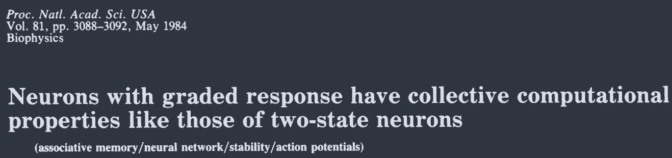
The same set of equations represents the resistively connected network of electrical amplifiers sketched in Fig. 2. It appears more complicated than the description of the neural system because the electrical problem of providing inhibition and excitation requires an additional inverting amplifier and a negative signal wire. The magnitude of $T_{ij}$ is $1/R_{ij}$, where $R_{ij}$ is the resistor connecting the output of $j$ to the input line $i$, while the sign of $T_{ij}$ is determined by the choice of the positive or negative output of amplifier $j$ at the connection site. $R_{i}$ is now
$$ \frac{1}{R_{i}} = \frac{1}{\rho_{i}} + \sum_{j}\frac{1}{R_{ij}} $$
where $\rho_{i}$ is the input resistance of amplifier $i$. $C_{i}$ is the total input capacitance of the amplifier $i$ and its associated input lead. We presume the output impedance of the amplifiers is negligible. These simplifications result in Eq. 5 being appropriate also for the network of Fig. 2.
同一组方程表示图 2 中草图所示的电阻连接的电子放大器网络。它看起来比神经系统的描述更复杂,因为提供抑制和兴奋的电气问题需要一个额外的反相放大器和一个负信号线。$T_{ij}$ 的大小是 $1/R_{ij}$,其中 $R_{ij}$ 是将 $j$ 的输出连接到输入线 $i$ 的电阻,而 $T_{ij}$ 的符号由放大器 $j$ 在连接点处选择正输出或负输出决定。$R_{i}$ 现在是
$$ \frac{1}{R_{i}} = \frac{1}{\rho_{i}} + \sum_{j}\frac{1}{R_{ij}} $$
其中 $\rho_{i}$ 是放大器 $i$ 的输入电阻。$C_{i}$ 是放大器 $i$ 及其相关输入引线的总输入电容。我们假设放大器的输出阻抗可以忽略不计。这些简化使得方程 5 也适用于图 2 的网络。
An electrical circuit that corresponds to Eq. 5 when the amplifiers are fast. The input capacitance and resistances are not drawn. A particularly simple special case can have all positive $T_{ij}$ of the same strength and no negative $T_{ij}$ and replaces the array of negative wires with a single negative feedback amplifier sending a common output to each “neuron.”
当放大器快速工作时,与公式 5 相对应的电路。输入电容和电阻未画出。一个特别简单的特例是,所有正向 $T_{ij}$ 的强度相同,而没有负向 $T_{ij}$,用一个向每个 “神经元” 发送共同输出的负反馈放大器来取代负向导线阵列。
Consider the quantity
$$ E = -\frac{1}{2}\sum_{i}\sum_{j}T_{ij}V_{i}V_{j} + \sum_{i}\frac{1}{R_{i}}\int_{0}^{V_{i}}g_{i}^{-1}(V)\mathrm{d}V + \sum_{i}I_{i}V_{i} $$
Its time derivative for a symmetric $T$ is
$$ \frac{\mathrm{d}E}{\mathrm{d}t} = -\sum_{i}\frac{\mathrm{d}V_{i}}{\mathrm{d}t}\left(\sum_{j}T_{ij}V_{j} - \frac{u_{i}}{R_{i}} + I_{i}\right). $$
The parenthesis is the right-hand side of Eq. 5, so
$$ \frac{\mathrm{d}E}{\mathrm{d}t} = -\sum C_{i}\frac{\mathrm{d}V_{i}}{\mathrm{d}t}\frac{\mathrm{d}u_{i}}{\mathrm{d}t} = -\sum C_{i}g_{i}^{-1\prime}(V_{i})\left(\frac{\mathrm{d}V_{i}}{\mathrm{d}t}\right)^{2}. $$
Since $g_{i}^{-1}(V_{i})$ is a monotone increasing function and $C_{i}$ is positive, each term in this sum is nonnegative. Therefore
$$ \frac{\mathrm{d}E}{\mathrm{d}t} \leq 0,\frac{\mathrm{d}E}{\mathrm{d}t} = 0\rightarrow \frac{\mathrm{d}V_{i}}{\mathrm{d}t} = 0\space\text{for all}\space i. $$
Together with the boundedness of $E$, Eq. 10 shows that the time evolution of the system is a motion in state space that seeks out minima in $E$ and comes to a stop at such points. $E$ is a Liapunov function for the system.
考虑量
$$ E = -\frac{1}{2}\sum_{i}\sum_{j}T_{ij}V_{i}V_{j} + \sum_{i}\frac{1}{R_{i}}\int_{0}^{V_{i}}g_{i}^{-1}(V)\mathrm{d}V + \sum_{i}I_{i}V_{i} $$
对于对称 $T$,它的时间导数是
$$ \frac{\mathrm{d}E}{\mathrm{d}t} = -\sum_{i}\frac{\mathrm{d}V_{i}}{\mathrm{d}t}\left(\sum_{j}T_{ij}V_{j} - \frac{u_{i}}{R_{i}} + I_{i}\right). $$
括号内是方程 5 的右侧,因此
$$ \frac{\mathrm{d}E}{\mathrm{d}t} = -\sum C_{i}\frac{\mathrm{d}V_{i}}{\mathrm{d}t}\frac{\mathrm{d}u_{i}}{\mathrm{d}t} = -\sum C_{i}g_{i}^{-1\prime}(V_{i})\left(\frac{\mathrm{d}V_{i}}{\mathrm{d}t}\right)^{2}. $$
由于 $g_{i}^{-1}(V_{i})$ 是单调递增函数且 $C_{i}$ 为正,因此该和中的每一项都是非负的。因此
$$ \frac{\mathrm{d}E}{\mathrm{d}t} \leq 0,\frac{\mathrm{d}E}{\mathrm{d}t} = 0\rightarrow \frac{\mathrm{d}V_{i}}{\mathrm{d}t} = 0\space\text{for all}\space i. $$
结合 $E$ 的有界性,方程 10 显示系统的时间演化是在状态空间中寻找 $E$ 的极小值并在这些点停止的运动。$E$ 是系统的 Liapunov 函数。
This deterministic model has the same flow properties in its continuous space that the stochastic model does in its discrete space. It can therefore be used in CAM or any other computational task for which an energy function is essential. We expect that the qualitative effects of disorganized or organized anti-symmetric parts of $T_{ij}$ should have similar effects on the CAM operation of the new’ and old system. The new computational behaviors (such as learning sequences) that can be produced by antisymmetric contributions to $T_{ij}$ within the stochastic model will also hold for the deterministic continuous model. Anecdotal support for these assertions comes from unpublished work of John Platt (California Institute of Technology) solving Eq. 5 on a computer with some random $T_{ij}$ removed from an otherwise symmetric $T$, and from experimental work of John Lambe (Jet Propulsion Laboratory), David Feinstein (California Institute of Technology), and Platt generating sequences of states by using an antisymmetric part of $T$ in a real circuit of a six “neurons” (personal communications).
该确定性模型在其连续空间中具有与随机模型在其离散空间中相同的流动特性。因此,它可以用于 CAM 或任何其他需要能量函数的计算任务。我们预计,$T_{ij}$ 的无组织或有组织的反对称部分的定性效应应该对新旧系统的 CAM 操作产生类似的影响。通过在随机模型中对 $T_{ij}$ 进行反对称贡献所产生的新计算行为(如学习序列)也适用于确定性的连续模型。对这些断言的轶事支持来自 John Platt(加州理工学院)的未发表工作,他在计算机上求解方程 5,并从一个本来是对称的 $T$ 中移除了一些随机 $T_{ij}$,以及 John Lambe(喷气推进实验室)、David Feinstein(加州理工学院)和 Platt 的实验工作,他们通过在一个由六个 “神经元” 组成的真实电路中使用 $T$ 的反对称部分生成状态序列(个人通信)。
Relation Between the Stable States of the Two Models
For a given $T$, the stable states of the continuous system have a simple correspondence with the stable states of the stochastic system. We will work with a slightly simplified instance of the general equations to put a minimum of mathematics in the way of seeing the correspondence. The same basic idea carries over, with more arithmetic, to the general case.
对于给定的 $T$,连续系统的稳定状态与随机系统的稳定状态有一个简单的对应关系。我们将使用一般方程的一个稍微简化的实例,以尽量减少数学方面的障碍,从而看到这种对应关系。相同的基本思想可以通过更多的算术运算推广到一般情况。
Consider the case in which $V_{i}^{0}<0<V_{i}^{1}$ for all $i$. Then the zero of voltage for each $V_{i}$ can be chosen such that $g_{i}(0) = 0$ for all $i$. Because the values of asymptotes are totally unimportant in all that follows, we will simplify notation by taking them as $\pm 1$ for all $i$. The second simplification is to treat the case in which $I_{i} = 0$ for all $i$. Finally, while the continuous case has an energy function with self-connections $T_{ii}$, the discrete case need not, so $T_{ii}=0$ will be assumed for the following analysis.
考虑 $V_{i}^{0}<0<V_{i}^{1}$ 对所有 $i$ 的情况。然后可以选择每个 $V_{i}$ 的电压零点,使得 $g_{i}(0) = 0$ 对所有 $i$ 成立。由于渐近线的值在接下来的所有内容中都是完全不重要的,我们将通过将它们简化为对所有 $i$ 取 $\pm 1$ 来简化符号。第二个简化是处理 $I_{i} = 0$ 对所有 $i$ 的情况。最后,虽然连续情况有一个具有自连接 $T_{ii}$ 的能量函数,但离散情况不需要,因此在以下分析中将假设 $T_{ii}=0$。
This continuous system has for symmetric $T$ the underlying energy function
$$ E = -\frac{1}{2}\sum_{i}\sum_{j\neq i}T_{ij}V_{i}V_{j} + \sum\frac{1}{R_{i}}\int_{0}^{V_{i}}g_{i}^{-1}(V)\mathrm{d}V. $$
对于对称的 $T$,这个连续系统的基本能量函数为
$$ E = -\frac{1}{2}\sum_{i}\sum_{j\neq i}T_{ij}V_{i}V_{j} + \sum\frac{1}{R_{i}}\int_{0}^{V_{i}}g_{i}^{-1}(V)\mathrm{d}V. $$
Where are the maxima and minima of the first term of Eq. 11 in the domain of the hypercube $-1\leq V_{i}\leq 1$ for all $i$? In the usual case, all extrema lie at corners of the $N$-dimensional hypercube space. [In the pathological case that $T$ is a positive or negative definite matrix, an extrermum is also possible in the interior of the space. This is not the case for information storage matrices of the usual type.]
在对所有 $i$ 的超立方体 $-1\leq V_{i}\leq 1$ 的领域中,方程 11 的第一项的最大值和最小值在哪里?在通常情况下,所有极值都位于 $N$ 维超立方体空间的角落处。[在病态情况下,如果 $T$ 是正定或负定矩阵,极值也可能出现在空间的内部。这不是通常类型的信息存储矩阵的情况。]
The discrete, stochastic algorithm searches for minimal states at the corners of the hypercube-corners that are lower than adjacent corners. Since $E$ is a linear function of a single $V_{i}$ along any cube edge, the energy minima (or maxima) of
$$ E = -\frac{1}{2}\sum_{i}\sum_{j\neq i}T_{ij}V_{i}V_{j} $$
for the discrete space $V_{i} = \pm 1$ are exactly the same corners as the energy maxima and minima for the continuous case $-1\leq V_{i}\leq 1$.
离散的随机算法在超立方体的角落处搜索最小状态——这些角落比相邻的角落更低。由于 $E$ 沿任何立方体边缘是单个 $V_{i}$ 的线性函数,因此对于离散空间 $V_{i} = \pm 1$,
The second term in Eq. 11 alters the overall picture somewhat. To understand that alteration most easily, the gain $g$ can be scaled, replacing
$$ V_{i} = g_{i}(u_{i}) \text{ by } V_{i} = g_{i}(\lambda u_{i}) $$
and
$$ u_{i} = g_{i}^{-1}(V_{i})\text{ by } u_{i} = \frac{1}{\lambda}g_{i}^{-1}(V_{i}) $$
This scaling changes the steepness of the sigmoid gain curve without altering the output asymptotes, as indicated in Fig. lb. $g_{i}(x)$ now represents a standard form in which the scale factor $\lambda = 1$ corresponds to a standard gain, $\lambda\gg 1$ to a system with very high gain and step-like gain curve, and $\lambda$ small corresponds to a low gain and flat sigmoid curve (Fig. lb). The second term in $E$ is now
$$ +\frac{1}{\lambda}\sum_{i}\frac{1}{R_{i}}\int_{0}^{V_{i}}g_{i}^{-1}(V)\mathrm{d}V. $$
The integral is zero for $V_{i} = 0$ and positive otherwise, getting very large as $V_{i}$ approaches $\pm 1$ because of the slowness with which $g(V)$ approaches its asymptotes (Fig. 1d). However, in the high-gain limit $\lambda\rightarrow \infty$ this second term becomes negligible, and the locations of the maxima and minima of the full energy expression become the same as that of Eq. 12 or Eq. 3 in the absence of inputs and zero thresholds. The only stable points of the very high gain, continuous, deterministic system therefore correspond to the stable points of the stochastic system.
方程 11 中的第二项稍微改变了整体情况。为了最容易理解这种变化,可以缩放增益,替换
$$ V_{i} = g_{i}(u_{i}) \text{ 以 } V_{i} = g_{i}(\lambda u_{i}) $$
和
$$ u_{i} = g_{i}^{-1}(V_{i})\text{ 以 } u_{i} = \frac{1}{\lambda}g_{i}^{-1}(V_{i}) $$
这种缩放改变了西格玛增益曲线的陡峭度,而不改变输出渐近线,如图 1b 所示。$g_{i}(x)$ 现在表示一个标准形式,其中比例因子 $\lambda = 1$ 对应于标准增益,$\lambda\gg 1$ 对应于具有非常高增益和阶跃状增益曲线的系统,而 $\lambda$ 小对应于低增益和平坦的西格玛曲线(图 1b)。$E$ 中的第二项现在是
$$ +\frac{1}{\lambda}\sum_{i}\frac{1}{R_{i}}\int_{0}^{V_{i}}g_{i}^{-1}(V)\mathrm{d}V. $$
当 $V_{i} = 0$ 时,积分为零,否则为正,并且当 $V_{i}$ 接近 $\pm 1$ 时变得非常大,因为 $g(V)$ 接近其渐近线的速度很慢(图 1d)。然而,在高增益极限 $\lambda\rightarrow \infty$ 下,这第二项变得可以忽略不计,并且完整能量表达式的最大值和最小值的位置与方程 12 或方程 3 在没有输入和零阈值的情况下的位置相同。因此,非常高增益的连续确定性系统的唯一稳定点对应于随机系统的稳定点。
For large but finite $\lambda$, the second term in Eq. 11 begins to contribute. The form of $g_{i}(V_{i})$ leads to a large positive contribution near all surfaces, edges, and corners of the hypercube while it still contributes negligibly far from the surfaces. This leads to an energy surface that still has its maxima at corners but the minima become displaced slightly toward the interior of the space. As $\lambda$ decreases, each minimum moves further inward. As $\lambda$ is further decreased minima disappear one at a time, when the topology of the energy surface makes a minimum and a saddle point coalesce. Ultimately, for very small $\lambda$, the second term in Eq. 11 dominates, and the only minimum is at $V_{i} = 0$. When the gain is large enough that there are many minima, each is associated with a well-defined minimum of the infinite gain case-as the gain is increased, each minimum will move until it reaches a particular cube corner when $\lambda\rightarrow \infty$. The same kind of mapping relation holds in general between the continuous deterministic system with sigmoid response curves and the stochastic model.
对于大但有限的 $\lambda$,方程 11 中的第二项开始起作用。$g_{i}(V_{i})$ 的形式导致在超立方体的所有表面、边缘和角落附近有一个大的正贡献,而在远离表面时仍然贡献可以忽略不计。这导致了一个能量表面,其最大值仍然位于角落,但最小值稍微向空间内部偏移。随着 $\lambda$ 的减小,每个最小值进一步向内移动。当能量表面的拓扑使得一个最小值和一个鞍点合并时,随着 $\lambda$ 的进一步减小,最小值一个接一个地消失。最终,对于非常小的 $\lambda$,方程 11 中的第二项占主导地位,唯一的最小值在 $V_{i} = 0$ 处。当增益足够大以至于存在许多最小值时,每个最小值都与无限增益情况下的一个明确定义的最小值相关联——随着增益的增加,每个最小值将移动,直到在 $\lambda\rightarrow \infty$ 时达到一个特定的立方体角落。在具有西格玛响应曲线的连续确定性系统与随机模型之间通常也存在同样类型的映射关系。
An energy contour map for a two-neuron (or two operational amplifier) system with two stable states is illustrated in Fig. 3. The two axes are the outputs of the two amplifiers. The upper left and lower right corners are stable minima for infinite gain, and the minima are displaced inward by the finite gain.
图 3 展示了具有两种稳定状态的双神经元(或双运算放大器)系统的能量等值线图。两条轴线是两个放大器的输出。左上角和右下角是无限增益时的稳定极小值,极小值因有限增益而向内移动。

FIG. 3. An energy contour map for a two-neuron, two-stablestate system. The ordinate and abscissa are the outputs of the two neurons. Stable states are located near the lower left and upper right corners, and unstable extrema at the other two corners. The arrows show the motion of the state from Eq. 5. This motion is not in general perpendicular to the energy contours. The system parameters are $T_{12} = T_{21} = 1$, $\lambda = 1.4$, and $g(u) = (2/\pi)\tan^{-1} (\pi\lambda u/2)$. Energy contours are $0.449$, $0.156$, $0.017$, $-0.003$, $-0.023$, and $-0.041$.
图 3. 一个双神经元、双稳定状态系统的能量等高线图。纵坐标和横坐标是两个神经元的输出。稳定状态位于左下角和右上角附近,不稳定的极值位于其他两个角落。箭头显示了方程 5 中状态的运动。这种运动通常不垂直于能量等高线。系统参数为 $T_{12} = T_{21} = 1$,$\lambda = 1.4$,且 $g(u) = (2/\pi)\tan^{-1} (\pi\lambda u/2)$。能量等高线分别为 $0.449$,$0.156$,$0.017$,$-0.003$,$-0.023$ 和 $-0.041$。
There are many general theorems about stability in networks of differential equations representing chemistry, circuits, and biology. The importance of this simple symmetric system is not merely its stability, but the fact that the correspondence with a discrete system lends it a special relation to elementary computational devices and concepts.
关于表示化学、电路和生物学的微分方程网络的稳定性,有许多一般定理。这个简单对称系统的重要性不仅在于它的稳定性,还在于它与离散系统的对应关系使其与基本计算设备和概念具有特殊的联系。
Discussion
Real neurons and real amplifiers have graded, continuous outputs as a function of their inputs (or sigmoid input-output curves of finite steepness) rather than steplike, two-state response curves. Our original stochastic model of CAM and other collective properties of assemblies of neurons was based on two-state neurons. A continuous, deterministic neuron network of interconnected neurons with graded responses has been analyzed in the previous two sections. It functions as a CAM in precisely the same collective way as did the original stochastic model of CAM. A set of memories can be nonlocally stored in a matrix of synaptic (or resistive) interconnections ih such a way that particular memories can be reconstructed from a starting state’that gives partial information about one of them.
真实的神经元和真实的放大器具有随其输入变化的分级、连续输出(或有限陡峭度的西格玛输入-输出曲线),而不是阶跃状的两态响应曲线。我们最初的 CAM 随机模型以及神经元集合的其他集体属性是基于两态神经元的。前两节分析了一个具有分级响应的互连神经元的连续确定性神经网络。它以与原始 CAM 随机模型完全相同的集体方式作为 CAM 运行。一组记忆可以非局部地存储在这样的突触(或电阻)互连矩阵中,以便可以从提供部分信息的起始状态重建特定记忆。
The convergence of the neuronal state of the continuous, deterministic model to its stable states (memories) is based on the existence of an energy function that directs the flow in state space. Such a function can be constructed in the continuous, deterministic model when $T$ is symmetric, just as was the case for the original stochastic model with two-state neurons. Other interesting uses and interpretations of the behaviors of the original model based on the existence of an underlying energy function will also hold for the continuous (“graded response”) model.
连续确定性模型的神经元状态收敛到其稳定状态(记忆)是基于存在一个能量函数,该函数指导状态空间中的流动。当 $T$ 是对称时,可以在连续确定性模型中构造这样的函数,就像原始的两态神经元随机模型的情况一样。基于存在基本能量函数的原始模型行为的其他有趣用途和解释也适用于连续(“分级响应”)模型。
A direct correspondence between the stable states of the two models was shown. For steep response curves (high gain) there is a 1:1 correspondence between the memories of the two models. When the response is less steep (lower gain) the continuous-response model can have fewer stable states than the stochastic model with the same $T$ matrix, but the existing stable states will still correspond to particular stable states of the stochastic model. This simple correspondence is possible because of the quadratic form of the interaction between different neurons in the energy function. More complicated energy functions, which have occasionally been used in constraint satisfaction problems, may have in addition stable states within the interior of the domain of state space in the continuous model which have no correspondence within the discrete two-state model.
两个模型的稳定状态之间显示了直接对应关系。对于陡峭的响应曲线(高增益),两个模型的记忆之间存在 1:1 的对应关系。当响应不那么陡峭(较低增益)时,连续响应模型可能具有比具有相同 $T$ 矩阵的随机模型更少的稳定状态,但现有的稳定状态仍然对应于随机模型的特定稳定状态。这种简单的对应关系是可能的,因为能量函数中不同神经元之间相互作用的二次形式。更复杂的能量函数,有时在约束满足问题中使用,可能在连续模型的状态空间域内部还有稳定状态,这些稳定状态在离散两态模型中没有对应关系。
This analysis indicates that a real circuit of operational amplifiers, capacitors, and resistors should be able to operate as a CAM, reconstructing the stable states that have been designed into $T$. As long as $T$ is symmetric and the amplifiers are fast compared with the characteristic RC time of the input network, the system will converge to stable states and cannot oscillate or display chaotic behavior. While the symmetry of the network is essential to the mathematics, a pragmatic view indicates that approximate symmetry will suffice, as was experimentally shown in the stochastic model. Equivalence of the gain curves and input capacitance of the amplifiers is not needed. For high-gain systems, the stable states of the real circuit will be exactly those predicted by the stochastic model.
该分析表明,一个由运算放大器、电容器和电阻器组成的真实电路应该能够作为 CAM 运行,重建已设计到 $T$ 中的稳定状态。只要 $T$ 是对称的,并且放大器相对于输入网络的特征 RC 时间足够快,系统将收敛到稳定状态,并且不会振荡或显示混沌行为。虽然网络的对称性对于数学是必不可少的,但务实的观点表明,近似对称性就足够了,正如在随机模型中实验所示。放大器的增益曲线和输入电容的等效性不是必需的。对于高增益系统,真实电路的稳定状态将完全符合随机模型的预测。
Neuronal and electromagnetic signals have finite propagation velocities. A neural circuit that is to operate in the mode described must have propagation delays that are considerably shorter than the RC or chemical integration time of the network. The same must be true for the slowness of amplifier response in the case of the electrical circuit.
神经元和电磁信号具有有限的传播速度。要以所描述的模式运行的神经电路必须具有比网络的 RC 或化学积分时间短得多的传播延迟。对于电路中的放大器响应的缓慢性也是如此。
The continuous model supplements, rather than replaces, the original stochastic description. The important properties of the original model are not due to its simplifications, but come from the general structure lying behind the model. Because the original model is very efficient to simulate on a digital computer, it will often be more practical to develop ideas and simulations on that model even when use on biological neurons or analog circuits is intended. The interesting collective properties transcend the 0-1 stochastic simplifications.
连续模型补充了原始的随机描述,而不是取代它。原始模型的重要属性不是由于其简化,而是来自模型背后的总体结构。由于原始模型在数字计算机上非常高效,因此即使打算在生物神经元或模拟电路上使用它,通常也更实用在该模型上开发想法和模拟。有趣的集体属性超越了 0-1 随机简化。
Neurons often communicate through action potentials. The output of such neurons consists of a series of sharp spikes having a mean frequency (when averaged over a short time) that is described by the input-output relation of Fig.1a. In addition, the delivery of transmitter at a synapse is quantized in vesicles. Thus Eq. 5 can be only an equation for the behavior of a neural network neglecting the quantal noise due to action potentials and the releases of discrete vesicles. Because the system operates by moving downhill on an energy surface, the injection of a small amount of quantal noise will not greatly change the minimum-seeking behavior.
神经元通常通过动作电位进行通信。这些神经元的输出由一系列尖锐的脉冲组成,其平均频率(在短时间内平均)由图 1a 的输入-输出关系描述。此外,突触处的递质传递是以囊泡的形式量化的。因此,方程 5 只能是一个神经网络行为的方程,忽略了由于动作电位和离散囊泡释放引起的噪声。由于系统通过在能量表面上向下移动来运行,因此注入少量噪声不会大大改变寻求最小值的行为。
Eq.5 has a generalization to include action potentials. Let all neurons have the same gain curves $g(u)$, input capacitance $C$, input impedance $R$, and maximum firing rate $F$. Let $g(u)$ have asymptotes 0 and 1. When a neuron has an input $u$, it is presumed to produce action potentials $V_{0}\delta(t - t_{\text{firing}})$ in a stochastic fashion with a probability $Fg(u)$ of producing an action potential per unit time. This stochastic view preserves the basic idea of the input signal being transformed into a firing rate but does not allow precise timing of individual action potentials. A synapse with strength $T_{ij}$ will deliver a quantal charge $V_{0}T_{ij}$ to the input capacitance of neuron $i$ when neuron $j$ produces an action potential. Let $P(u_{1}, u_{2}, \cdots, u_{i},\cdots, u_{N},t)\mathrm{d}u_{1}, \mathrm{d}u_{2}, …, \mathrm{d}u_{N}$ be the probability that input potential 1 has the value $u_{1},\cdots$ The evolution of the state of the network is described by
$$ \frac{\partial P}{\partial t} = \sum_{i}\frac{1}{RC}\frac{\partial(u_{i}P)}{\partial u_{i}} + \sum_{j} Fg(u_{j})[-P+P(u_{1}-T_{1j}V_{0}/C,\cdots,u_{i}-T_{ij}V_{0}/C,\cdots)]. $$
If $V_{0}$ is small, the term in brackets can be expanded in a Taylor series, yielding
$$ \frac{\partial P}{\partial t} = \sum_{i}\frac{1}{RC}\frac{\partial (u_{i}P)}{\partial u_{i}} - \sum_{j}\frac{\partial \dot{P}}{\partial u_{i}}\frac{V_{0}F}{C}\sum_{i}T_{ij}g(u_{j}) + \frac{V_{0}^{2}F}{2C^{2}}\sum_{ijk}g(u_{k})T_{ik}T_{jk}\frac{\partial^{2}P}{\partial u_{i}\partial u_{j}}. $$
In the limit as $V_{0}\rightarrow 0$, $F\rightarrow \infty$ such that $FV_{0} =$ constant, the second derivative term can be omitted. This simplification has the solutions that are identical to those of the continuous, deterministic model, namely
$$ P = \prod\delta(u_{i}-u_{i}(t)) $$
where $u_{i}(t)$ obeys Eq. 5.
方程 5 有一个包含动作电位的推广。让所有神经元具有相同的增益曲线 $g(u)$、输入电容 $C$、输入阻抗 $R$ 和最大发放率 $F$。让 $g(u)$ 具有渐近线 0 和 1。当神经元具有输入 $u$ 时,假设它以随机方式产生动作电位 $V_{0}\delta(t - t_{\text{firing}})$,每单位时间产生动作电位的概率为 $Fg(u)$。这种随机观点保留了输入信号被转换为发放率的基本思想,但不允许单个动作电位的精确时序。具有强度 $T_{ij}$ 的突触将在神经元 $j$ 产生动作电位时向神经元 $i$ 的输入电容传递量化电荷 $V_{0}T_{ij}$。令 $P(u_{1}, u_{2}, \cdots, u_{i},\cdots, u_{N},t)\mathrm{d}u_{1}, \mathrm{d}u_{2}, …, \mathrm{d}u_{N}$ 为输入电位 1 具有值 $u_{1},\cdots$ 的概率。网络状态的演化由下式描述
$$ \frac{\partial P}{\partial t} = \sum_{i}\frac{1}{RC}\frac{\partial(u_{i}P)}{\partial u_{i}} + \sum_{j} Fg(u_{j})[-P+P(u_{1}-T_{1j}V_{0}/C,\cdots,u_{i}-T_{ij}V_{0}/C,\cdots)]. $$
如果 $V_{0}$ 很小,则括号内的项可以展开成泰勒级数,得到
$$ \frac{\partial P}{\partial t} = \sum_{i}\frac{1}{RC}\frac{\partial (u_{i}P)}{\partial u_{i}} - \sum_{j}\frac{\partial \dot{P}}{\partial u_{i}}\frac{V_{0}F}{C}\sum_{i}T_{ij}g(u_{j}) + \frac{V_{0}^{2}F}{2C^{2}}\sum_{ijk}g(u_{k})T_{ik}T_{jk}\frac{\partial^{2}P}{\partial u_{i}\partial u_{j}}. $$
在 $V_{0}\rightarrow 0$,$F\rightarrow \infty$ 且 $FV_{0} =$ 常数的极限下,可以省略二阶导数项。这种简化的解与连续确定性模型的解相同,即
$$ P = \prod\delta(u_{i}-u_{i}(t)) $$
其中 $u_{i}(t)$ 遵循方程 5。
In the model, stochastic noise from the action potentials disappears in this limit and the continuous model of Eq. 5 is recovered. The second derivative term in Eq. 16 produces noise in the system in the same fashion that diffusion produces broadening in mobility-diffusion equations. These equations permit the study of the effects of action potential noise on the continuous, deterministic system. Questions such as the duration of stability of nominal stable states of the continuous, deterministic model Eq. 5 in the presence of action potential noise should be directly answerable from analysis or simulations of Eq. 15 or 16. Unfortunately the steady-state solution of this problem is not equivalent to a thermal distribution-while Eq. 15 is a master equation, it does not have detailed balance even in the high-gain limit, and the quantal noise is not characterized by a temperature.
在该模型中,来自动作电位的随机噪声在此极限下消失,并且恢复了方程 5 的连续模型。方程 16 中的二阶导数项以与扩散在迁移-扩散方程中产生展宽相同的方式在系统中产生噪声。这些方程允许研究动作电位噪声对连续确定性系统的影响。在存在动作电位噪声的情况下,连续确定性模型方程 5 的名义稳定状态的稳定持续时间等问题应该可以直接从方程 15 或 16 的分析或模拟中得到解答。不幸的是,这个问题的稳态解不等同于热分布——虽然方程 15 是一个主方程,但即使在高增益极限下它也没有详细平衡,并且量化噪声没有用温度来表征。