Abstract
Computational properties of use to biological organisms or to the construction of computers can emerge as collective properties of systems -having a large number of simple equivalent components (or neurons). The physical meaning ofcontent-addressable memory is described by an appropriate phase space flow of the state of a system. A model of such a system is given, based on aspects of neurobiology but readily adapted to integrated circuits. The collective properties of this model produce a content-addressable memory which correctly yields an entire memory from any subpart of sufficient size. The algorithm for the time evolution of the state of the system is based on asynchronous parallel processing. Additional emergent collective properties include some capacity for generalization, familiarity recognition, categorization, error correction, and time sequence retention. The collective properties are only weakly sensitive to details ofthe modeling or the failure of individual devices.
对生物有机体或计算机构造有用的计算特性,可以作为拥有大量简单等效组件(或神经元)的系统的集体特性而出现。内容可寻址记忆的物理意义可以用系统状态的适当相空间流来描述。本文给出了这样一个系统模型,该模型基于神经生物学的某些方面,但很容易适用于集成电路。这个模型的集体特性产生了一个内容可寻址存储器,它能正确地从任何足够大小的子部分产生整个存储器。系统状态的时间演化算法基于异步并行处理。其他出现的集体特性包括一定的概括能力、熟悉度识别能力、分类能力、纠错能力和时序保持能力。集体特性对建模细节或单个设备故障的敏感度很低。
Given the dynamical electrochemical properties ofneurons and their interconnections (synapses), we readily understand schemes that use a few neurons to obtain elementary useful biological behavior. Our understanding of such simple circuits in electronics allows us to plan larger and more complex circuits which are essential to large computers. Because evolution has no such plan, it becomes relevant to ask whether the ability of large collections of neurons to perform “computational” tasks may in part be a spontaneous collective consequence of having a large number of interacting simple neurons.
鉴于神经元及其相互连接(突触)的动态电化学特性,我们很容易理解使用少量神经元来获得基本有用的生物行为的方案。我们对电子学中这种简单电路的理解使我们能够设计更大更复杂的电路,这对于大型计算机来说是必不可少的。由于进化没有这样的计划,因此有必要问一下,大量神经元集合执行“计算”任务的能力是否在某种程度上是拥有大量相互作用的简单神经元的自发集体结果。
In physical systems made from a large number of simple elements, interactions among large numbers of elementary components yield collective phenomena such as the stable magnetic orientations and domains in a magnetic system or the vortex patterns in fluid flow. Do analogous collective phenomena in a system of simple interacting neurons have useful “computational” correlates? For example, are the stability of memories, the construction of categories of generalization, or time-sequential memory also emergent properties and collective in origin? This paper examines a new modeling ofthis old and fundamental question and shows that important computational properties spontaneously arise.
在由大量简单元素组成的物理系统中,大量基本组件之间的相互作用产生了集体现象,例如磁系统中的稳定磁取向和畴,或流体流动中的涡旋模式。简单相互作用神经元系统中是否存在类似的集体现象,并具有有用的“计算”相关性?例如,记忆的稳定性、概括类别的构建或时间序列记忆是否也是涌现属性且具有集体起源?本文考察了这一古老而基本问题的新建模,并表明重要的计算属性会自发出现。
All modeling is based on details, and the details of neuroanatomy and neural function are both myriad and incompletely known. In many physical systems, the nature of the emergent collective properties is insensitive to the details inserted in the model (e.g., collisions are essential to generate sound waves, but any reasonable interatomic force law will yield appropriate collisions). In the same spirit, I will seek collective properties that are robust against change in the model details.
所有建模都是基于细节的,而神经解剖学和神经功能的细节既繁多又不完全为人所知。在许多物理系统中,涌现的集体属性的性质对模型中插入的细节不敏感(例如,碰撞对于产生声波是必不可少的,但任何合理的原子间力定律都能产生适当的碰撞)。本着同样的精神,我将寻找对模型细节变化具有鲁棒性的集体属性。
The model could be readily implemented by integrated circuit hardware. The conclusions suggest the design of a delocalized content-addressable memory or categorizer using extensive asynchronous parallel processing.
该模型可以通过集成电路硬件轻松实现。结论表明,使用广泛的异步并行处理设计一个分散的内容可寻址存储器或分类器是可行的。
The general content-addressable memory of a physical system
Suppose that an item stored in memory is “H. A. Kramers & G. H. Wannier Phys. Rev. 60, 252 (1941).” A general contentaddressable memory would be capable of retrieving this entire memory item on the basis of sufficient partial information. The input "& Wannier, (1941)" might suffice. An ideal memory could deal with errors and retrieve this reference even from the input “Vannier, (1941)”. In computers, only relatively simple forms of content-addressable memory have been made in hardware. Sophisticated ideas like error correction in accessing information are usually introduced as software.
假设存储在内存中的一项是 “H. A. Kramers & G. H. Wannier Phys. Rev. 60, 252 (1941).” 一个通用的内容可寻址存储器能够基于足够的部分信息检索出整个存储项。输入 "& Wannier, (1941)" 可能就足够了。一个理想的存储器可以处理错误,甚至可以从输入 “Vannier, (1941)” 中检索出这个参考。在计算机中,只有相对简单形式的内容可寻址存储器被硬件实现。像访问信息中的纠错这样复杂的想法通常作为软件引入。
There are classes of physical systems whose spontaneous behavior can be used as a form of general (and error-correcting) content-addressable memory. Consider the time evolution of a physical system that can be described by a set of general coordinates. A point in state space then represents the instantaneous condition of the system. This state space may be either continuous or discrete (as in the case of $N$ Ising spins).
存在一些物理系统,其自发行为可以用作一种通用(和纠错)内容可寻址存储器。考虑一个可以用一组广义坐标描述的物理系统的时间演化。状态空间中的一个点代表系统的瞬时状态。这个状态空间可以是连续的,也可以是离散的(如 $N$ 个 Ising 自旋的情况)。
The equations ofmotion ofthe system describe a flow in state space. Various classes offlow patterns are possible, but the systems of use for memory particularly include those that flow toward locally stable points from anywhere within regions around those points. A particle with frictional damping moving in a potential well with two minima exemplifies such a dynamics.
系统的运动方程描述了状态空间中的流动。各种类型的流动模式都是可能的,但用于存储的系统特别包括那些从这些点周围的任何地方流向局部稳定点的系统。在具有两个极小值的势阱中运动并具有摩擦阻尼的粒子就是这种动力学的一个例子。
If the flow is not completely deterministic, the description is more complicated. In the two-well problems above, if the frictional force is characterized by atemperature, it must also produce a random driving force. The limit points become small limiting regions, and the stability becomes not absolute. But as long as the stochastic effects are small, the essence of local stable points remains.
如果流动不是完全确定性的,那么描述就会更复杂。在上述双阱问题中,如果摩擦力由温度表征,它还必须产生一个随机驱动力。极限点变成了小的极限区域,稳定性也不是绝对的。但只要随机效应很小,局部稳定点的本质仍然存在。
Consider a physical system described by many coordinates $X_1\cdots X_N$, the components of a state vector $X$. Let the system have locally stable limit points $X_a, X_b,\cdots$. Then, if the system is started sufficiently near any $X_a$, as at $X = X_a + \Delta$, it will proceed in time until $X\approx X_a$. We can regard the information stored in the system as the vectors $X_a, X_b, \cdots$. The starting point $X = X_a + \Delta$ represents a partial knowledge of the item $X_a$, and the system then generates the total information $X_{a}$.
考虑一个由许多坐标 $X_1\cdots X_N$ 描述的物理系统,这些坐标是状态向量 $X$ 的分量。让系统具有局部稳定的极限点 $X_a, X_b,\cdots$。那么,如果系统从足够接近任何 $X_a$ 的地方开始,例如在 $X = X_a + \Delta$ 处,它将随着时间的推移直到 $X\approx X_a$。我们可以将存储在系统中的信息视为向量 $X_a, X_b, \cdots$。起始点 $X = X_a + \Delta$ 代表对项 $X_a$ 的部分了解,然后系统生成完整的信息 $X_{a}$。
Any physical system whose dynamics in phase space is dominated by a substantial number of locally stable states to which it is attracted can therefore be regarded as a general contentaddressable memory. The physical system will be a potentially useful memory if, in addition, any prescribed set of states can readily be made the stable states of the system.
因此,任何在相空间中由大量局部稳定状态主导其动力学并被吸引到这些状态的物理系统都可以被视为一种通用的内容可寻址存储器。如果还可以轻松地将任何预定的一组状态设为系统的稳定状态,那么该物理系统将成为一个潜在有用的存储器。
The model system
The processing devices will be called neurons. Each neuron $i$ has two states like those of McCullough and Pitts: $V_i = 0$(“not firing”) and $V_i = 1$ (“firing at maximum rate”). When neuron $i$ has a connection made to it from neuron $j$, the strength of connection is defined as $T_{ij}$. (Nonconnected neurons have $T_{ij} = 0$.) The instantaneous state of the system is specified by listing the $N$ values of $V_i$, so it is represented by a binary word of $N$ bits.
处理设备将被称为神经元。每个神经元 $i$ 有两个状态,类似于 McCullough 和 Pitts 的状态:$V_i = 0$(“不发火”)和 $V_i = 1$(“以最大速率发火”)。当神经元 $i$ 与神经元 $j$ 建立连接时,连接的强度定义为 $T_{ij}$。(未连接的神经元具有 $T_{ij} = 0$。)系统的瞬时状态通过列出 $N$ 个 $V_i$ 的值来指定,因此它表示为一个由 $N$ 位组成的二进制字。
The state changes in time according to the following algorithm. For each neuron $i$ there is a fixed threshold $U_i$. Each neuron $i$ readjusts its state randomly in time but with a mean attempt rate $W$, setting
$$ \begin{equation*} \begin{aligned} \begin{array}{c}V_{i}\rightarrow 1\\V_{i}\rightarrow 0\end{array}\quad\text{if}\quad\sum_{j\neq i}T_{ij}V_{j}\begin{array}{c} >U_{i}\\ <U_{i}\end{array} \end{aligned} \end{equation*} $$
Thus, each neuron randomly and asynchronously evaluates whether it is above or below threshold and readjusts accordingly. (Unless otherwise stated, we choose $U_i = 0$.)
神经元 $i$ 的状态根据以下算法随时间变化。对于每个神经元 $i$,都有一个固定的阈值 $U_i$。每个神经元 $i$ 以平均尝试速率 $W$ 随机地调整其状态,设置
$$ \begin{equation*} \begin{aligned} \begin{array}{c}V_{i}\rightarrow 1\\V_{i}\rightarrow 0\end{array}\quad\text{if}\quad\sum_{j\neq i}T_{ij}V_{j}\begin{array}{c} >U_{i}\\ <U_{i}\end{array} \end{aligned} \end{equation*} $$
因此,每个神经元随机且异步地评估它是高于还是低于阈值,并相应地进行调整。(除非另有说明,我们选择 $U_i = 0$。)
Although this model has superficial similarities to the Perceptron the essential differences are responsible for the new results. First, Perceptrons were modeled chiefly with neural connections in a “forward” direction $A\rightarrow B \rightarrow C \rightarrow D$. The analysis of networks with strong backward coupling $A\rightleftarrows B\rightleftarrows C\rightleftarrows A$ proved intractable. All our interesting results arise as consequences of the strong back-coupling. Second, Perceptron studies usually made a random net ofneurons deal directly with a real physical world and did not ask the questions essential to finding the more abstract emergent computational properties. Finally, Perceptron modeling required synchronous neurons like a conventional digital computer. There is no evidence for such global synchrony and, given the delays of nerve signal propagation, there would be no way to use global synchrony effectively. Chiefly computational properties which can exist in spite of asynchrony have interesting implications in biology.
虽然这个模型在表面上与感知器有相似之处,但本质上的差异导致了新的结果。首先,感知器主要以“前向”方向的神经连接进行建模 $A\rightarrow B \rightarrow C \rightarrow D$。具有强反向耦合 $A\rightleftarrows B\rightleftarrows C\rightleftarrows A$ 的网络分析被证明是难以处理的。我们所有有趣的结果都是强反向耦合的结果。其次,感知器研究通常让一个随机神经元网络直接处理一个真实的物理世界,并没有提出发现更抽象的涌现计算属性所必需的问题。最后,感知器建模需要像传统数字计算机一样同步的神经元。没有证据表明存在这种全局同步,并且考虑到神经信号传播的延迟,也没有办法有效地利用全局同步。主要是那些尽管存在异步性但仍然可以存在的计算属性在生物学中具有有趣的意义。
The information storage algorithm
Suppose we wish to store the set of states $V^{s}, s = 1\cdots n$. We use the storage prescription
$$ T_{ij} = \sum_{s}(2V_{i}^{s}-1)(2V_{j}^{s}-1) $$
but with $T_{ii} = 0$. From this definition
$$ \sum_{j}T_{ij}V_{j}^{s^{\prime}} = \sum_{s}(2V_{i}^{s}-1)\left[\sum_{j}V_{j}^{s^{\prime}}(2V_{j}^{s}-1)\right] \equiv H_{j}^{s^{\prime}}. $$
The mean value of the bracketed term in Eq. 3 is $0$ unless $s = s^{\prime}$, for which the mean is $N/2$. This pseudoorthogonality yields
$$ \sum_{j}T_{ij}V_{j}^{s^{\prime}}\equiv \langle H_{i}^{s^{\prime}}\rangle \approx (2V_{i}^{s^{\prime}}-1)N/2. $$
and is positive if $V_{i}^{s^{\prime}} = 1$ and negative if $V_{i}^{s^{\prime}} = 0$. Except for the noise coming from the $s\neq s^{\prime}$ terms, the stored state would always be stable under our processing algorithm.
假设我们希望存储状态集 $V^{s}, s = 1\cdots n$。我们使用存储处方
$$ T_{ij} = \sum_{s}(2V_{i}^{s}-1)(2V_{j}^{s}-1) $$
但 $T_{ii} = 0$。根据这个定义
$$ \sum_{j}T_{ij}V_{j}^{s^{\prime}} = \sum_{s}(2V_{i}^{s}-1)\left[\sum_{j}V_{j}^{s^{\prime}}(2V_{j}^{s}-1)\right] \equiv H_{j}^{s^{\prime}}. $$
括号中项的平均值在 $s \neq s^{\prime}$ 时为 $0$,而在 $s = s^{\prime}$ 时平均值为 $N/2$。这种伪正交性产生了
$$ \sum_{j}T_{ij}V_{j}^{s^{\prime}}\equiv \langle H_{i}^{s^{\prime}}\rangle \approx (2V_{i}^{s^{\prime}}-1)N/2. $$
并且当 $V_{i}^{s^{\prime}} = 1$ 时为正,当 $V_{i}^{s^{\prime}} = 0$ 时为负。除了来自 $s\neq s^{\prime}$ 项的噪声外,存储的状态在我们的处理算法下总是稳定的。
Such matrices $T_{ij}$ have been used in theories of linear associative nets to produce an output pattern from a paired input stimulus, $S_1 \rightarrow O_1$. A second association $S_2 \rightarrow O_2$ can be simultaneously stored in the same network. But the confusing stimulus $0.6 S_1 + 0.4 O_2$ will produce a generally meaningless mixed output $0.6 O_1 + 0.4 O_2$. Our model, in contrast, will use its strong nonlinearity to make choices, produce categories, and regenerate information and, with high probability, will generate the output $O_1$ from such a confusing mixed stimulus.
这样的矩阵 $T_{ij}$ 已被用于线性联想网络的理论中,以从配对的输入刺激中产生输出模式,$S_1 \rightarrow O_1$。第二个关联 $S_2 \rightarrow O_2$ 可以同时存储在同一个网络中。但混淆的刺激 $0.6 S_1 + 0.4 O_2$ 通常会产生一个毫无意义的混合输出 $0.6 O_1 + 0.4 O_2$。相比之下,我们的模型将利用其强非线性来做出选择、产生类别和再生信息,并且很可能会从这样一个混淆的混合刺激中生成输出 $O_1$。
A linear associative net must be connected in a complex way with an external nonlinear logic processor in order to yield true computation. Complex circuitry is easy to plan but more difficult to discuss in evolutionary terms. In contrast, our model obtains its emergent computational properties from simple properties of many cells rather than circuitry.
线性联想网络必须与外部非线性逻辑处理器以复杂的方式连接,才能产生真正的计算。复杂的电路设计很容易,但在进化论方面更难讨论。相比之下,我们的模型从许多细胞的简单属性中获得其涌现的计算属性,而不是电路。
The biological interpretation of the model
Most neurons are capable of generating a train of action potentials-propagating pulses of electrochemical activity-when the average potential across their membrane is held well above its normal resting value. The mean rate at which action potentials are generated is a smooth function of the mean membrane potential, having the general form shown in Fig. 1.
当神经元膜上的平均电位远高于其正常静息值时,大多数神经元都能产生一连串动作电位–电化学活动的传播脉冲。动作电位产生的平均速率是平均膜电位的平滑函数,其一般形式如图 1 所示。
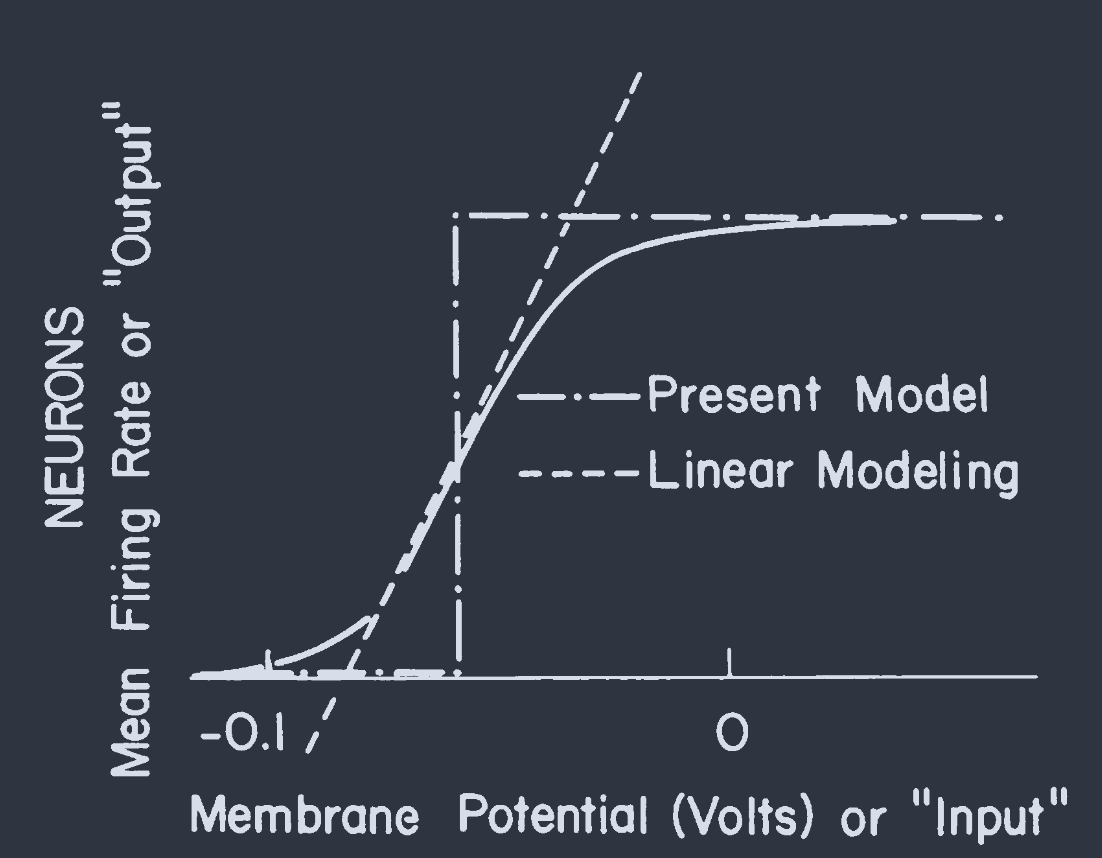
FIG. 1. Firing rate versus membrane voltage for a typical neuron (solid line), dropping to 0 for large negative potentials and saturating for positive potentials. The broken lines show approximations used in modeling.
图1显示了典型神经元的放电频率与膜电压的关系(实线),在大负电位下降为0,在正电位下饱和。虚线显示了建模中使用的近似。
The biological information sent to other neurons often lies in a short-time average of the firing rate. When this is so, one can neglect the details of individual action potentials and regard Fig. 1 as a smooth input-output relationship. [Parallel pathways carrying the same information would enhance the ability of the system to extract a short-term average firing rate.]
发送到其他神经元的生物信息通常存在于放电率的短时间平均值中。当情况如此时,可以忽略单个动作电位的细节,并将图 1 视为一个平滑的输入输出关系。[携带相同信息的并行路径将增强系统提取短期平均放电频率的能力。]
A study of emergent collective effects and spontaneous computation must necessarily focus on the nonlinearity of the input-output relationship. The essence of computation is nonlinear logical operations. The particle interactions that produce true collective effects in particle dynamics come from a nonlinear dependence of forces on positions of the particles. Whereas linear associative networks have emphasized the linear central region of Fig. 1, we will replace the input-output relationship by the dot-dash step. Those neurons whose operation is dominantly linear merely provide a pathway of communication between nonlinear neurons. Thus, we consider a network of “on or off” neurons, granting that some of the interconnections may be by way of neurons operating in the linear regime.
对突发集体效应和自发计算的研究,必须关注输入-输出关系的非线性。计算的本质是非线性逻辑运算。粒子动力学中产生真正集体效应的粒子相互作用来自于力对粒子位置的非线性依赖。线性关联网络强调的是图 1 中的线性中心区域,而我们将用点-虚线步骤取代输入-输出关系。那些以线性操作为主的神经元只是提供了非线性神经元之间的交流途径。因此,我们考虑的是一个由 “开或关” 神经元组成的网络,当然其中的一些相互连接可能是通过在线性机制下工作的神经元实现的。
Delays in synaptic transmission (of partially stochastic character) and in the transmission of impulses along axons and dendrites produce a delay between the input of a neuron and the generation of an effective output. All such delays have been modeled by a single parameter, the stochastic mean processing time $1/W$.
突触传递(具有部分随机特性)以及沿轴突和树突传递冲动的延迟会导致神经元输入与产生有效输出之间的延迟。所有这些延迟都被建模为一个参数,即随机平均处理时间 $1/W$。
The input to a particular neuron arises from the current leaks of the synapses to that neuron, which influence the cell mean potential. The synapses are activated by arriving action potentials. The input signal to a cell $i$ can be taken to be
$$ \sum_{j}T_{ij}V_{j} $$
where $T_{ij}$ represents the effectiveness of a synapse. Fig. 1 thus becomes an input-output relationship for a neuron.
特定神经元的输入来自于突触的电流泄漏,这些泄漏影响细胞的平均电位。突触由到达的动作电位激活。对细胞 $i$ 的输入信号可以表示为
$$ \sum_{j}T_{ij}V_{j} $$
其中 $T_{ij}$ 代表突触的有效性。因此,图 1 成为神经元的输入-输出关系。
Little, Shaw, and Roney have developed ideas on the collective functioning ofneural nets based on “on/off” neurons and synchronous processing. However, in their model the relative timing of action potential spikes was central and resulted in reverberating action potential trains. Our model and theirs have limited formal similarity, although there may be connections at a deeper level.
Little、Shaw 和 Roney 基于“开/关”神经元和同步处理,发展了关于神经网络集体功能的思想。然而,在他们的模型中,动作电位峰值的相对时机是核心,并导致了回响的动作电位序列。我们的模型与他们的模型在形式上有一定的相似性,尽管在更深层次上可能存在联系。
Most modeling of neural learning networks has been based on synapses of a general type described by Hebb and Eccles. The essential ingredient is the modification of $T_{ij}$ by correlations like
$$ \Delta T_{ij} = [V_{i}(t)V_{j}(t)]_{\text{average}} $$
where the average is some appropriate calculation over past history. Decay in time and effects of $[V_{i}(t)]_{\text{avg}}$ or $[V_{j}(t)]_{\text{avg}}$ are also allowed. Model networks with such synapses can construct the associative $T_{ij}$ of Eq. 2. We will therefore initially assume that such a $T_{ij}$ has been produced by previous experience (or inheritance). The Hebbian property need not reside in single synapses; small groups of cells which produce such a net effect would suffice.
大多数神经学习网络的建模都是基于 Hebb 和 Eccles 描述的一般类型的突触。基本成分是通过类似以下的相关性来修改 $T_{ij}$
$$ \Delta T_{ij} = [V_{i}(t)V_{j}(t)]_{\text{average}} $$
其中平均值是对过去历史进行的一些适当计算。时间衰减和 $[V_{i}(t)]_{\text{avg}}$ 或 $[V_{j}(t)]_{\text{avg}}$ 的影响也是允许的。具有这种突触的模型网络可以构建方程 2 中的关联 $T_{ij}$。因此,我们将最初假设这样的 $T_{ij}$ 是由先前的经验(或遗传)产生的。Hebbian 属性不必存在于单个突触中,产生这种净效应的小组细胞就足够了。
The network of cells we describe performs an abstract calculation and, for applications, the inputs should be appropriately coded. In visual processing, for example, feature extraction should previously have been done. The present modeling might then be related to how an entity or Gestalt is remembered or categorized on the basis of inputs representing a collection of its features.
我们描述的细胞网络执行抽象计算,对于应用来说,输入应该被适当地编码。例如,在视觉处理中,应该先进行特征提取。然后,当前的建模可能与如何基于代表其特征集合的输入来记忆或分类一个实体或格式塔有关。
Studies of the collective behaviors of the model
The model has stable limit points. Consider the special case $T_{ij} = T_{ji}$, and define
$$ E = -\frac{1}{2}\sum_{i,j\neq i}T_{ij}V_{i}V_{j} $$
$\Delta E$ due to $\Delta V_{i}$ is given by
$$ \Delta E = -\Delta V_{i}\sum_{j\neq i^{\prime}}T_{ij}V_{j} $$
Thus, the algorithm for altering $V_{i}$ causes $E$ to be a monotonically decreasing function. State changes will continue until a least (local) $E$ is reached. This case is isomorphic with an Ising model. $T_{ij}$ provides the role ofthe exchange coupling, and there is also an external local field at each site. When $T_{ij}$ is symmetric but has a random character (the spin glass) there are known to be many (locally) stable states.
该模型具有稳定的极限点。考虑特殊情况 $T_{ij} = T_{ji}$,并定义
$$ E = -\frac{1}{2}\sum_{i,j\neq i}T_{ij}V_{i}V_{j} $$
由于 $\Delta V_{i}$ 引起的 $\Delta E$ 由下式给出
$$ \Delta E = -\Delta V_{i}\sum_{j\neq i^{\prime}}T_{ij}V_{j} $$
因此,改变 $V_{i}$ 的算法使得 $E$ 成为单调递减函数。状态变化将持续直到达到最小(局部)$E$。这种情况与 Ising 模型同构。$T_{ij}$ 提供了交换耦合的作用,并且在每个位置还有一个外部局部场。当 $T_{ij}$ 是对称的但具有随机特性(自旋玻璃)时,已知存在许多(局部)稳定状态。
Monte Carlo calculations were made on systems of $N = 30$ and $N = 100$, to examine the effect of removing the $T_{ij} = T_{ji}$ restriction. Each element of $T_{ij}$ was chosen as a random number between $-1$ and $1$. The neural architecture of typical cortical regions and also of simple ganglia of invertebrates suggests the importance of $100-10,000$ cells with intense mutual interconnections in elementary processing, so our scale of $N$ is slightly small.
进行了 $N = 30$ 和 $N = 100$ 系统的蒙特卡洛计算,以检查去除 $T_{ij} = T_{ji}$ 限制的影响。$T_{ij}$ 的每个元素都被选择为介于 $-1$ 和 $1$ 之间的随机数。典型皮层区域以及无脊椎动物简单神经节的神经结构表明,在基本处理过程中,$100-10,000$ 个细胞具有强烈的相互连接,因此我们的 $N$ 规模略小。
The dynamics algorithm was initiated from randomly chosen initial starting configurations. For $N = 30$ the system never displayed an ergodic wandering through state space. Within a time of about $4/W$ it settled into limiting behaviors, the commonest being a stable state. When $50$ trials were examined for a particular such random matrix, all would result in one of two or three end states. A few stable states thus collect the flow from most of the initial state space. A simple cycle also occurred occasionally-for example, $\cdots A\rightarrow B\rightarrow A\rightarrow B\cdots$.
对于 $N = 30$,系统从未显示出在状态空间中的遍历游荡。在大约 $4/W$ 的时间内,它会稳定下来,最常见的是一个稳定状态。当检查了某个特定随机矩阵的 $50$ 次试验时,所有试验都将导致两个或三个最终状态之一。因此,一些简单的循环也偶尔发生,例如,$\cdots A\rightarrow B\rightarrow A\rightarrow B\cdots$。
The third behavior seen was chaotic wandering in a small region of state space. The Hamming distance between two binary states $A$ and $B$ is defined as the number of places in which the digits are different. The chaotic wandering occurred within a short Hamming distance of one particular state. Statistics were done on the probability $p_{i}$ of the occurrence of a state in a time of wandering around this minimum, and an entropic measure of the available states $M$ was taken
$$ \ln{M} = -\sum p_{i}\ln{p_{i}}. $$
A value of $M = 25$ was found for $N = 30$. The flow in phase space produced by this model algorithm has the properties necessary for a physical content-addressable memory whether or not $T_{ij}$ is symmetric.
第三种行为是在状态空间的小区域内的混沌游荡。定义两个二进制状态 $A$ 和 $B$ 之间的 Hamming 距离为数字不同的位置数。混沌游荡发生在离某个特定状态很近的 Hamming 距离内。对在围绕该极小值游荡一段时间内状态出现的概率 $p_{i}$ 进行了统计,并采用了可用状态的熵度量 $M$
$$ \ln{M} = -\sum p_{i}\ln{p_{i}} $$
对于 $N = 30$,发现 $M = 25$。无论 $T_{ij}$ 是否对称,该模型算法在相空间中产生的流动都具有作为物理内容可寻址存储器所必需的属性。
Simulations with $N = 100$ were much slower and not quantitatively pursued. They showed qualitative similarity to $N = 30$.
$N = 100$ 的模拟速度较慢,未进行定量研究。它们在定性上与 $N = 30$ 显示出相似性。
Why should stable limit points or regions persist when $T_{ij} \neq T_{ji}$? If the algorithm at some time changes $V_{i}$ from $0$ to $1$ or vice versa, the change of the energy defined in Eq. 7 can be split into two terms, one of which is always negative. The second is identical if $T_{ij}$ is symmetric and is “stochastic” with mean 0 if $T_{ij}$ and $T_{ji}$ are randomly chosen. The algorithm for $T_{ij} \neq T_{ji}$, therefore changes $E$ in a fashion similar to the way $E$ would change in time for a symmetric $T_{ij}$ but with an algorithm corresponding to a finite temperature.
为什么当 $T_{ij} \neq T_{ji}$ 时,稳定的极限点或区域仍然存在?如果算法在某个时间将 $V_{i}$ 从 $0$ 改变为 $1$ 或反之亦然,则方程 7 中定义的能量变化可以分为两项,其中一项总是负的。如果 $T_{ij}$ 是对称的,第二项是相同的;如果 $T_{ij}$ 和 $T_{ji}$ 是随机选择的,则其 “随机” 且平均值为 0。因此,$T_{ij} \neq T_{ji}$ 的算法以类似于对称 $T_{ij}$ 随时间变化的方式改变 $E$,但算法对应于有限温度。
About $0.15 N$ states can be simultaneously remembered before error in recall is severe. Computer modeling of memory storage according to Eq. 2 was carried out for $N = 30$ and $N = 100$. $n$ random memory states were chosen and the corresponding $T_{ij}$ was generated. If a nervous system preprocessed signals for efficient storage, the preprocessed information would appear random (e.g., the coding sequences of DNA have a random character). The random memory vectors thus simulate efficiently encoded real information, as well as representing our ignorance. The system was started at each assigned nominal memory state, and the state was allowed to evolve until stationary.
在回忆错误严重之前,大约 $0.15 N$ 个状态可以同时被记住。根据方程 2 进行了 $N = 30$ 和 $N = 100$ 的存储记忆的计算机建模。选择了 $n$ 个随机记忆状态,并生成了相应的 $T_{ij}$。如果神经系统对信号进行预处理以实现高效存储,则预处理的信息将呈现随机性(例如,DNA 的编码序列具有随机特性)。因此,随机记忆向量有效地模拟了经过高效编码的真实信息,同时也代表了我们的无知。系统从每个指定的名义记忆状态开始,并允许状态演变直到稳定。
Typical results are shown in Fig. 2. The statistics are averages over both the states in a given matrix and different matrices. With $n = 5$, the assigned memory states are almost always stable (and exactly recallable). For $n = 15$, about half of the nominally remembered states evolved to stable states with less than $5$ errors, but the rest evolved to states quite different from the starting points.
典型结果如图 2 所示。统计数据是对给定矩阵中的状态和不同矩阵的平均值。对于 $n = 5$,指定的记忆状态几乎总是稳定的(并且可以精确回忆)。对于 $n = 15$,大约一半的名义记忆状态演变为错误少于 $5$ 的稳定状态,但其余的演变为与起始点完全不同的状态。
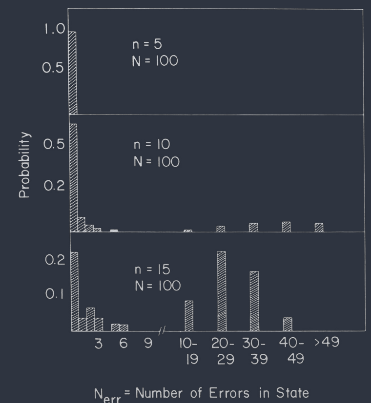
FIG. 2. The probability distribution of the occurrence of errors in the location of the stable states obtained from nominally assigned memories.
图 2 显示了从名义上分配的记忆中获得的稳定状态位置错误发生的概率分布。
These results can be understood from an analysis of the effect of the noise terms. In Eq. 3, $H_{i}^{s^{\prime}}$ is the “effective field” on neuron $i$ when the state of the system is $s^{\prime}$, one of the nominal memory states. The expectation value of this sum, Eq. 4, is $\pm N/2$ as appropriate. The $s\neq s^{\prime}$ summation in Eq. 2 contributes no mean, but has a rms noise of $[(n - 1)N/2]^{1/2}2\equiv \sigma$. For $nN$ large, this noise is approximately Gaussian and the probability of an error in a single particular bit of a particular memory will be
$$ P = \frac{1}{\sqrt{2\pi\sigma^{2}}}\int_{N/2}^{\infty}e^{-x^{2}/2\sigma^{2}}dx. $$
For the case $n = 10$, $N = 100$, $P = 0.0091$, the probability that a state had no errors in its $100$ bits should be about $e^{-0.91} \approx 0.40$. In the simulation of Fig. 2, the experimental number was $0.6$.
这些结果可以从对噪声项影响的分析中理解。在方程 3 中,当系统状态为 $s^{\prime}$(名义记忆状态之一)时,$H_{i}^{s^{\prime}}$ 是神经元 $i$ 上的“有效场”。该和式的期望值(方程 4)为 $\pm N/2$。方程 2 中的 $s\neq s^{\prime}$ 求和没有贡献均值,但具有均方根噪声 $[(n - 1)N/2]^{1/2}2\equiv \sigma$。对于大的 $nN$,这种噪声近似为高斯分布,特定记忆的单个位发生错误的概率为
$$ P = \frac{1}{\sqrt{2\pi\sigma^{2}}}\int_{N/2}^{\infty}e^{-x^{2}/2\sigma^{2}}dx. $$
对于 $n = 10$,$N = 100$ 的情况,$P = 0.0091$,一个状态在其 $100$ 位中没有错误的概率应约为 $e^{-0.91} \approx 0.40$。在图 2 的模拟中,实验值为 $0.6$。
The theoretical scaling of $n$ with $N$ at fixed $P$ was demonstrated in the simulations going between $N = 30$ and $N = 100$. The experimental results of half the memories being well retained at $n = 0.15 N$ and the rest badly retained is expected to be true for all large $N$. The information storage at a given level of accuracy can be increased by a factor of $2$ by a judicious choice of individual neuron thresholds. This choice is equivalent to using variables $\mu_{i} = \pm 1$, $T_{ij} = \sum_{s}\mu_{i}^{s}\mu_{j}^{s}$, and a threshold level of $0$.
在固定 $P$ 下,$n$ 随 $N$ 的理论标度在 $N = 30$ 和 $N = 100$ 之间的模拟中得到了证明。在 $n = 0.15 N$ 时,一半的记忆被很好地保留,其余的记忆被严重保留,这一实验结果预计对所有大的 $N$ 都是正确的。通过明智地选择单个神经元阈值,可以将给定精度水平下的信息存储增加一个因子 $2$。这种选择等同于使用变量 $\mu_{i} = \pm 1$,$T_{ij} = \sum_{s}\mu_{i}^{s}\mu_{j}^{s}$,以及阈值水平为 $0$。
Given some arbitrary starting state, what is the resulting final state (or statistically, states)? To study this, evolutions from randomly chosen initial states were tabulated for $N = 30$ and $n = 5$. From the (inessential) symmetry of the algorithm, if $(101110\cdots)$ is an assigned stable state, $(010001\cdots)$ is also stable. Therefore, the matrices had $10$ nominal stable states. Approximately 85% of the trials ended in assigned memories, and 10% ended in stable states of no obvious meaning. An ambiguous 5% landed in stable states very near assigned memories. There was a range of a factor of 20 of the likelihood of finding these 10 states.
给定一些任意的起始状态,最终状态(或统计上,状态)是什么?为了研究这一点,对 $N = 30$ 和 $n = 5$ 的随机选择初始状态的演变进行了统计。由于算法的(非本质)对称性,如果 $(101110\cdots)$ 是一个指定的稳定状态,那么 $(010001\cdots)$ 也是稳定的。因此,矩阵有 $10$ 个名义稳定状态。大约 85% 的试验以指定的记忆结束,10% 以没有明显意义的稳定状态结束。大约 5% 的不明确状态落在非常接近指定记忆的稳定状态中。找到这 10 个状态的可能性存在一个因素为 20 的范围。
The algorithm leads to memories near the starting state. For $N = 30$, $n = 5$, partially random starting states were generated by random modification of known memories. The probability that the final state was that closest to the initial state was studied as a function of the distance between the initial state and the nearest memory state. For distance $\leq 5$, the nearest state was reached more than 90% of the time. Beyond that distance, the probability fell off smoothly, dropping to a level of $0.2$ (2 times random chance) for a distance of 12.
该算法导致记忆接近起始状态。对于 $N = 30$,$n = 5$,通过随机修改已知记忆生成部分随机起始状态。研究了最终状态是最接近初始状态的概率,作为初始状态与最近记忆状态之间距离的函数。对于距离 $\leq 5$,最接近的状态超过 90% 的时间被达到。超过该距离后,概率平稳下降,在距离为 12 时降至 $0.2$(是随机机会的两倍)。
The phase space flow is apparently dominated by attractors which are the nominally assigned memories, each of which dominates a substantial region around it. The flow is not entirely deterministic, and the system responds to an ambiguous starting state by a statistical choice between the memory states it most resembles.
相空间流显然由吸引子主导,这些吸引子是名义上分配的记忆,每个记忆都主导着其周围的一个重要区域。流动并非完全确定性,系统通过在它最像的记忆状态之间进行统计选择来响应模糊的起始状态。
Were it desired to use such a system in an $S_{i}$-based content addressable memory, the algorithm should be used and modified to hold the known bits of information while letting the others adjust.
如果希望在基于 $S_{i}$ 的内容可寻址存储器中使用这样的系统,则应使用该算法并进行修改,以保持已知的信息位,同时让其他位进行调整。
The model was studied by using a “clipped” $T_{ij}$, replacing $T_{ij}$ in Eq. 3 by $\pm 1$, the algebraic sign of $T_{ij}$. The purposes were to examine the necessity of a linear synapse supposition (by making a highly nonlinear one) and to examine the efficiency of storage. Only $N(N/2)$ bits of information can possibly be stored in this symmetric matrix. Experimentally, for $N = 100$, $n = 9$, the level of errors was similar to that for the ordinary algorithm at $n = 12$. The signal-to-noise ratio can be evaluated analytically for this clipped algorithm and is reduced by a factor of $(2/\pi)^{1/2}$ compared with the unclipped case. For a fixed error probability, the number of memories must be reduced by $2/\pi$.
通过使用 “简化” $T_{ij}$ 研究了该模型,在方程 3 中将 $T_{ij}$ 替换为 $T_{ij}$ 的代数符号 $\pm 1$。目的在于通过制作一个高度非线性的突触来检查线性突触假设的必要性,并检查存储效率。在这个对称矩阵中,最多只能存储 $N(N/2)$ 位信息。实验上,对于 $N = 100$,$n = 9$,错误水平与普通算法在 $n = 12$ 时的错误水平相似。可以对这个裁剪算法进行信噪比的解析评估,并且与未裁剪情况相比,信噪比降低了一个因子 $(2/\pi)^{1/2}$。对于固定的错误概率,记忆数量必须减少 $2/\pi$。
With the $\mu$ algorithm and the clipped $T_{ij}$, both analysis and modeling showed that the maximal information stored for $N = 100$ occurred at about $n = 13$. Some errors were present, and the Shannon information stored corresponded to about $N(N/8)$ bits.
使用 $\mu$ 算法和裁剪的 $T_{ij}$,分析和建模都显示,对于 $N = 100$,存储的最大信息量约在 $n = 13$ 时出现。存在一些错误,存储的 Shannon 信息对应于大约 $N(N/8)$ bit。
New memories can be continually added to $T_{ij}$. The addition of new memories beyond the capacity overloads the system and makes all memory states irretrievable unless there is a provision for forgetting old memories.
可以不断地将新记忆添加到 $T_{ij}$ 中。超出容量的新记忆的添加会使系统过载,并且除非有忘记旧记忆的规定,否则所有记忆状态都无法检索。
The saturation of the possible size of $T_{ij}$ will itself cause forgetting. Let the possible values of $T_{ij}$ be $0, \pm 1, \pm 2, \pm 3$, and be freely incremented within this range. If $T_{ij} = 3$, a next increment of +1 would be ignored and a next increment of $-1$ would reduce $T_{ij}$ to $2$. When $T_{ij}$ is so constructed, only the recent memory states are retained, with a slightly increased noise level. Memories from the distant past are no longer stable. How far into the past are states remembered depends on the digitizing depth of $T_{ij}$, and $0, \cdots,\pm 3$ is an appropriate level for $N = 100$. Other schemes can be used to keep too many memories from being simultaneously written, but this particular one is attractive because it requires no delicate balances and is a consequence of natural hardware.
$T_{ij}$ 可能的大小饱和本身会导致遗忘。让 $T_{ij}$ 的可能值为 $0, \pm 1, \pm 2, \pm 3$,并在此范围内自由递增。如果 $T_{ij} = 3$,下一个 $+1$ 的增量将被忽略,下一个 $-1$ 的增量将使 $T_{ij}$ 降至 $2$。当 $T_{ij}$ 这样构造时,只保留最近的记忆状态,噪声水平略有增加。来自遥远过去的记忆不再稳定。记忆状态被记住的时间取决于 $T_{ij}$ 的数字化深度,而 $0, \cdots,\pm 3$ 是 $N = 100$ 的适当水平。可以使用其他方案来防止同时写入过多的记忆,但这个特定的方案很有吸引力,因为它不需要微妙的平衡,并且是自然硬件的结果。
Real neurons need not make synapses both of $i\rightarrow j$ and $j\rightarrow i$. Particular synapses are restricted to one sign of output. We therefore asked whether $T_{ij} = T_{ji}$ is important. Simulations were carried out with only one $ij$ connection: if $T_{ij}\neq 0$, $T_{ji} = 0$. The probability of making errors increased, but the algorithm continued to generate stable minima. A Gaussian noise description of the error rate shows that the signal-to-noise ratio for given $n$ and $N$ should be decreased by the factor $1/\sqrt{2}$, and the simulations were consistent with such a factor. This same analysis shows that the system generally fails in a “soft” fashion, with signal-to-noise ratio and error rate increasing slowly as more synapses fail.
真实的神经元不需要同时对 $i\rightarrow j$ 和 $j\rightarrow i$ 进行突触连接。特定的突触仅限于一种输出符号。因此,我们问是否 $T_{ij} = T_{ji}$ 很重要。进行了仅有一个 $ij$ 连接的模拟:如果 $T_{ij}\neq 0$,则 $T_{ji} = 0$。错误的概率增加了,但算法继续生成稳定的极小值。对错误率的高斯噪声描述表明,对于给定的 $n$ 和 $N$,信噪比应降低因子 $1/\sqrt{2}$,模拟结果与该因子一致。相同的分析表明,系统通常以“软”方式失败,随着更多突触失效,信噪比和错误率缓慢增加。
Memories too close to each other are confused and tend to merge. For $N = 100$, a pair ofrandom memories should be separated by $50\pm 5$ Hamming units. The case $N = 100$, $n = 8$, was studied with seven random memories and the eighth made up a Hamming distance of only $30$, $20$, or $10$ from one of the other seven memories. At a distance of $30$, both similar memories were usually stable. At a distance of $20$, the minima were usually distinct but displaced. At a distance of $10$, the minima were often fused.
过于接近的记忆会混淆并倾向于合并。对于 $N = 100$,一对随机记忆应相隔 $50\pm 5$ 个 Hamming 单位。研究了 $N = 100$,$n = 8$ 的情况,其中七个随机记忆,第八个与其他七个记忆之一的 Hamming 距离仅为 $30$、$20$ 或 $10$。在距离为 $30$ 时,两个相似的记忆通常是稳定的。在距离为 $20$ 时,极小值通常是不同的但被位移了。在距离为 $10$ 时,极小值经常融合在一起。
The algorithm categorizes initial states according to the similarity to memory states. With a threshold of $0$, the system behaves as a forced categorizer.
该算法根据与记忆状态的相似性对初始状态进行分类。使用 $0$ 的阈值时,系统表现为强制分类器。
The state $00000\cdots$ is always stable. For a threshold of $0$, this stable state is much higher in energy than the stored memory states and very seldom occurs. Adding a uniform threshold in the algorithm is equivalent to raising the effective energy of the stored memories compared to the $0000$ state, and $0000$ also becomes a likely stable state. The $0000$ state is then generated by any initial state that does not resemble adequately closely one of the assigned memories and represents positive recognition that the starting state is not familiar.
状态 $00000\cdots$ 总是稳定的。对于阈值为 $0$,这个稳定状态的能量远高于存储的记忆状态,并且很少发生。在算法中添加一个统一的阈值相当于提高了存储记忆的有效能量与 $0000$ 状态相比,并且 $0000$ 也成为一个可能的稳定状态。然后,任何不够接近地类似于指定记忆之一的初始状态都会生成 $0000$ 状态,并表示对起始状态不熟悉的积极识别。
Familiarity can be recognized by other means when the memory is drastically overloaded. We examined the case $N = 100$, $n = 500$, in which there is a memory overload of a factor of $25$. None of the memory states assigned were stable. The initial rate of processing of a starting state is defined as the number of neuron state readjustments that occur in a time $1/2W$. Familiar and unfamiliar states were distinguishable most of the time at this level of overload on the basis of the initial processing rate, which was faster for unfamiliar states. This kind of familiarity can only be read out of the system by a class of neurons or devices abstracting average properties of the processing group.
当记忆被大幅度超载时,可以通过其他方式识别熟悉度。我们检查了 $N = 100$,$n = 500$ 的情况,其中记忆超载了 $25$ 倍。在这种情况下,没有分配的记忆状态是稳定的。起始状态的初始处理速率定义为在时间 $1/2W$ 内发生的神经元状态重新调整的数量。在这种超载水平下,大多数时候可以根据初始处理速率区分熟悉和不熟悉的状态,不熟悉的状态处理速度更快。这种熟悉度只能通过一类神经元或设备从处理组中抽象出平均属性来读取系统。
For the cases so far considered, the expectation value of $T_{ij}$ was 0 for $i\neq j$. A set of memories can be stored with average correlations, and $\bar{T}_{ij} = C_{ij} \neq 0$ because there is a consistent internal correlation in the memories. If now a partial new state $X$ is stored
$$ \Delta T_{ij} = (2X_{i}-1)(2X_{j}-1)\quad i,j\leq k<N $$
using only $k$ of the neurons rather than $N$, an attempt to reconstruct it will generate a stable point for all $N$ neurons. The values of $X_{k+1}\cdots X_{N}$ that result will be determined primarily from the sign of
$$ \sum_{j=1}^{k}c_{ij}x_{j} $$
and $X$ is completed according to the mean correlations of the other memories. The most effective implementation of this capacity stores a large number of correlated matrices weakly followed by a normal storage of $X$.
到目前为止考虑的情况中,$i\neq j$ 时 $T_{ij}$ 的期望值为 0。一组记忆可以存储具有平均相关性的内容,并且 $\bar{T}_{ij} = C_{ij} \neq 0$,因为记忆中存在一致的内部相关性。如果现在存储一个部分新状态 $X$
$$ \Delta T_{ij} = (2X_{i}-1)(2X_{j}-1)\quad i,j\leq k<N $$
仅使用 $k$ 个神经元而不是 $N$,尝试重构它将为所有 $N$ 个神经元生成一个稳定点。结果的 $X_{k+1}\cdots X_{N}$ 的值将主要由以下的符号决定
$$ \sum_{j=1}^{k}c_{ij}x_{j} $$
并且 $X$ 根据其他记忆的平均相关性进行补全。这种容量的最有效实现是弱跟踪大量相关矩阵,然后正常存储 $X$。
A nonsymmetric $T_{ij}$ can lead to the possibility that a minimum will be only metastable and will be replaced in time by another minimum. Additional nonsymmetric terms which could be easily generated by a minor modification of Hebb synapses
$$ \Delta T_{ij} = A\sum_{s}(2V_{i}^{s+1}-1)(2V_{j}^{s}-1) $$
were added to $T_{ij}$. When $A$ was judiciously adjusted, the system would spend a while near $V_{s}$ and then leave and go to a point near $V_{s+1}$. But sequences longer than four states proved impossible to generate, and even these were not faithfully followed.
非对称的 $T_{ij}$ 可能导致一个极小值仅是亚稳态,并且随着时间的推移会被另一个极小值取代。通过对 Hebb 突触进行小幅修改,可以轻松生成的额外非对称项
$$ \Delta T_{ij} = A\sum_{s}(2V_{i}^{s+1}-1)(2V_{j}^{s}-1) $$
被添加到 $T_{ij}$ 中。当 $A$ 被明智地调整时,系统会在 $V_{s}$ 附近停留一段时间,然后离开并前往 $V_{s+1}$ 附近的点。但证明无法生成超过四个状态的序列,即使是这些状态也没有被忠实地跟随。
Discussion
In the model network each “neuron” has elementary properties, and the network has little structure. Nonetheless, collective computational properties spontaneously arose. Memories are retained as stable entities or Gestalts and can be correctly recalled from any reasonably sized subpart. Ambiguities are resolved on a statistical basis. Some capacity for generalization is present, and time ordering of memories can also be encoded. These properties follow from the nature of the flow in phase space produced by the processing algorithm, which does not appear to be strongly dependent on precise details of the modeling. This robustness suggests that similar effects will obtain even when more neurobiological details are added.
在模型网络中,每个 “神经元” 都具有基本属性,并且网络几乎没有结构。尽管如此,集体计算属性自发地出现了。记忆作为稳定的实体或格式塔被保留,并且可以从任何合理大小的子部分正确回忆出来。模糊性以统计为基础得到解决。存在一定的泛化能力,记忆的时间顺序也可以被编码。这些属性源于处理算法在相空间中产生的流动的性质,这似乎并不强烈依赖于建模的精确细节。这种鲁棒性表明,即使添加了更多神经生物学细节,也会获得类似的效果。
Much of the architecture of regions of the brains of higher animals must be made from a proliferation of simple local circuits with well-defined functions. The bridge between simple circuits and the complex computational properties of higher nervous systems may be the spontaneous emergence of new computational capabilities from the collective behavior of large numbers of simple processing elements.
高等动物大脑区域的大部分结构必须由大量具有明确定义功能的简单局部电路组成。简单电路与高级神经系统复杂计算属性之间的桥梁可能是大量简单处理单元的集体行为中自发出现的新计算能力。
Implementation of a similar model by using integrated circuits would lead to chips which are much less sensitive to element failure and soft-failure than are normal circuits. Such chips would be wasteful of gates but could be made many times larger than standard designs at a given yield. Their asynchronous parallel processing capability would provide rapid solutions to some special classes of computational problems.
通过使用集成电路实现类似的模型将导致芯片对元件故障和软故障的敏感性远低于普通电路。这些芯片在门电路方面可能比较浪费,但在给定的产量下可以比标准设计大很多倍。它们的异步并行处理能力将为某些特殊类别的计算问题提供快速解决方案。