Abstract
Coronal heating has been a long-standing conundrum in solar physics. Parker’s conjecture that spontaneous current singularities lead to nanoflares that heat the corona has been controversial. In ideal magnetohydrodynamics (MHD), can genuine current singularities emerge from a smooth 3D line-tied magnetic field? To numerically resolve this issue, the schemes employed must preserve magnetic topology exactly to avoid artificial reconnection in the presence of (nearly) singular current densities.
日冕加热是太阳物理学中一个长期存在的难题。Parker 关于自发电流奇点会导致加热日冕的纳米火花的猜想一直备受争议。在理想的磁流体力学(MHD)中,平滑的三维线束磁场能否产生真正的电流奇点?要在数值上解决这个问题,所采用的方案必须精确地保留磁拓扑结构,以避免在存在(近似)奇异电流密度的情况下出现人为的重新连接。
Structure-preserving numerical methods are favorable for mitigating numerical dissipation, and variational integration is a powerful machinery for deriving them. However, successful applications of variational integration to ideal MHD have been scarce. In this thesis, we develop variational integrators for ideal MHD in Lagrangian labeling by discretizing Newcomb’s Lagrangian on a moving mesh using discretized exterior calculus. With the built-in frozen-in equation, the schemes are free of artificial reconnection, hence optimal for studying current singularity formation.
保结构数值方法有利于减少数值耗散,而变分积分是推导这些方法的强大工具。然而,变分法在理想 MHD 中的成功应用还很少。在本论文中,我们通过使用离散化外部微积分对移动网格上的纽科姆拉格朗日进行离散化,为拉格朗日标注的理想 MHD 开发了变分积分器。由于内置了冻结方程,这些方案不存在人为重联,因此是研究当前奇点形成的最佳方案。
Using this method, we first study a fundamental prototype problem in 2D, the HahmKulsrud-Taylor (HKT) problem. It considers the effect of boundary perturbations on a 2D plasma magnetized by a sheared field, and its linear solution is singular. We find that with increasing resolution, the nonlinear solution converges to one with a current singularity. The same signature of current singularity is also identified in other 2D cases with more complex magnetic topologies, such as the coalescence instability of magnetic islands.
利用这种方法,我们首先研究了二维的一个基本原型问题,即 HahmKulsrud-Taylor(HKT)问题。它考虑了边界扰动对由剪切场磁化的二维等离子体的影响,其线性解是奇异的。我们发现,随着分辨率的提高,非线性解收敛到一个具有电流奇点的解。在其他具有更复杂磁拓扑结构的二维情况下,例如磁岛的聚合不稳定性,也发现了相同的电流奇点特征。
We then extend the HKT problem to 3D line-tied geometry, which models the solar corona by anchoring the field lines in the boundaries. The effect of such geometry is crucial in the controversy over Parker’s conjecture. The linear solution, which is singular in 2D, is found to be smooth. However, with finite amplitude, it can become pathological above a critical system length. The nonlinear solution turns out smooth for short systems. Nonetheless, the scaling of peak current density vs. system length suggests that the nonlinear solution may become singular at a finite length. With the results in hand, we cannot confirm or rule out this possibility conclusively, since we cannot obtain solutions with system lengths near the extrapolated critical value.
我们然后将 HKT 问题扩展到三维线束几何,通过将磁力线锚定在边界上来模拟太阳日冕。这种几何结构的影响在 Parker 猜想的争议中至关重要。发现在二维中是奇异的线性解是光滑的。然而,在有限幅度下,它可能在超过临界系统长度时变得病态。对于短系统,非线性解最终是光滑的。然而,峰值电流密度与系统长度的标度表明,非线性解可能在有限长度处变得奇异。根据现有结果,我们无法明确确认或排除这种可能性,因为我们无法获得接近外推临界值的系统长度的解。
Chapter 1: Introduction
The work in this thesis consists of two parts: the first is the development of a novel numerical method, variational integration for ideal magnetohydrodynamics (MHD); the second is to apply this method to studying a computationally challenging problem, formation of current singularities. This chapter serves the purpose of briefly surveying the background literatures for these two projects.
In Sec. 1.1, we identify how our method fits into the lively landscape of structure-preserving numerical methods (for plasma physics).
In Sec. 1.2, we review what has previously been accomplished on the problem of current singularity formation, in the contexts of both toroidal fusion plasmas and solar coronal heating, and overview what progress is made in this thesis. Readers that are primarily interested in the new results can safely skip this chapter and proceed to the subsequent ones, which are meant to be self-contained.
本论文的工作包括两个部分:第一部分是开发一种新颖的数值方法,即理想磁流体力学(MHD)的变分积分;第二部分是应用该方法研究一个计算上具有挑战性的问题,即电流奇点的形成。本章旨在简要回顾这两个项目的背景文献。
在第 1.1 节中,我们确定了我们的方法如何适应保结构数值方法(用于等离子体物理学)的活跃领域。
在第 1.2 节中,我们回顾了在环形聚变等离子体和太阳日冕加热的背景下,当前奇点形成问题上已经取得的成就,并概述了本论文取得的进展。主要对新结果感兴趣的读者可以安全地跳过本章,直接进入后续章节,这些章节旨在自成一体。
1.1 Structure-preserving numerical methods
Computation has become widely acknowledged as the third pillar of science. Still, the pursuit for better computational methods has never ceased. A specific motivation in the development of numerical methods for computational physics is to respect the physical properties of the original systems, which are often described in terms of conservation laws. In other words, it is preferable that the accumulation of the errors embedded in the numerical schemes do not violate the conservation laws of the systems. Otherwise, the fidelity of the numerical results is undermined, particularly in long-term simulations. For example, using the standard RungeKutta methods to simulate Hamiltonian systems (as simple as a pendulum) often results in coherent drifts in energy, which eventually become significant and make the solutions unphysical and unreliable.
计算已被公认为科学的第三大支柱。然而,对更好计算方法的追求从未停止。开发计算物理数值方法的一个具体动机是尊重原始系统的物理特性,而原始系统通常是用守恒定律来描述的。换句话说,数值方案中的误差累积最好不违反系统的守恒定律。否则,数值结果的保真度就会受到影响,特别是在长期模拟中。例如,使用标准 RungeKutta 方法模拟哈密顿系统(如钟摆一样简单)往往会导致能量的相干漂移,这种漂移最终会变得很明显,使求解变得不符合物理规律和不可靠。
Many have come up with various manipulations to enforce conservation laws for different systems when developing numerical schemes. The caveat with these manipulations is that they are often ad hoc and lack generality, and therefore can be troublesome to invent when the system is as complicated as many in plasma physics. In contrast, an alternative approach is to try to preserve the structures that underpin the conservation laws. It is difficult to explicitly define what structures exactly mean here, but within the scope of this thesis, the symmetry, geometry, and Hamiltonian structures, etc., of the systems all fall into this category. Numerical methods obtained in this manner often enjoy general applicability to a class of systems that share similar structures.
许多人在开发数值方案时,想出了各种操作来强制执行不同系统的守恒定律。这些操作的警告是它们通常是特设的,缺乏通用性,因此当系统像等离子体物理学中的许多系统一样复杂时,发明这些操作可能会很麻烦。相比之下,另一种方法是尝试保留支撑守恒定律的结构。在这里很难明确定义结构到底是什么意思,但在本论文的范围内,系统的对称性、几何和哈密顿结构等都属于这一类。以这种方式获得的数值方法通常适用于具有类似结构的一类系统。
Simplest examples of structure-preserving numerical methods are probably the Stormer-Verlet method and the leapfrog method for solving Hamilton’s equations, which had long been used before people realized that both methods are symplectic1 . Symplectic integrators have superior long-term energy behaviors for preserving the symplectic structures of the Hamiltonian systems (Hairer et al., 2006), and hence have become the standard methods in simulating many-body systems such as molecular or celestial dynamics.
保结构数值方法的最简单例子可能是用于求解哈密顿方程的 Störmer-Verlet 方法和跳跃法,这两种方法在被人们意识到它们都是辛方法之前就已经被广泛使用了。辛积分器在保持哈密顿系统的辛结构方面具有优越的长期能量行为(Hairer 等,2006),因此已成为模拟分子或天体动力学等多体系统的标准方法。
A popular and powerful machinery for deriving structure-preserving numerical methods is variational integration (Marsden & West, 2001). The idea is to discretize the Lagrangians, rather than equations of motion, of the systems, and then obtain numerical schemes from a discrete variational principle. These schemes can naturally inherit many of the structures and the consequent conservation laws of the original systems. For finite-dimensional systems with non-degenerate Lagrangians, it is proven that variational integrators are not only symplectic, but also momentum-preserving due to a discrete Noether’s theorem (Marsden & West, 2001). The St¨ormer-Verlet method, among many other symplectic integrators, can be derived variationally.
变分积分(Marsden & West,2001)是一种流行且强大的推导保结构数值方法的工具。其思想是对系统的拉格朗日量而不是运动方程进行离散化,然后从离散变分原理中获得数值方案。这些方案可以自然地继承原始系统的许多结构及其相应的守恒定律。对于具有非简并拉格朗日量的有限维系统,已经证明变分积分器不仅是辛的,而且由于离散诺特定理(Marsden & West,2001),它们也是动量守恒的。Störmer-Verlet 方法以及许多其他辛积分器都可以通过变分法推导出来。
However, life is not so easy for plasma physicists, as things get much more complicated as soon as electromagnetic fields are involved. To solve for the trajectory of a charged particle in a prescribed electromagnetic field, which is the simplest problem in plasma physics, the standard methods of symplectic or variational integration usually lead to schemes that are implicit and impractical. The most popular explicit method for this problem has been the Boris method (Boris, 1970) for its excellent long-term accuracy.
As Qin et al. (2013) recently showed, the underlying reason is that the Boris method preserves phase space volume, even though it is not symplectic. The Boris method had subsequently been generalized to volumepreserving methods with higher orders (He et al., 2015b, 2016a) and for relativistic dynamics (Zhang et al., 2015). Also, explicit symplectic (Zhang et al., 2016), explicit K-symplectic (He et al., 2017), and Lorentz covariant canonical symplectic methods (Wang et al., 2016) for the problem have been developed.
然而,对于等离子体物理学家来说,情况并非如此简单,因为一旦涉及电磁场,事情就会变得复杂得多。为了解决在规定的电磁场中带电粒子的轨迹问题,这是等离子体物理学中最简单的问题,辛或变分积分的标准方法通常会导致隐式且不实用的方案。该问题最流行的显式方法是 Boris 方法(Boris,1970),因为它具有出色的长期精度。
正如秦等人(2013)最近所展示的,Boris 方法的基本原因是它保持了相空间体积,尽管它不是辛的。随后,Boris 方法被推广到具有更高阶数的体积保持方法(He 等人,2015b,2016a)和相对论动力学(Zhang 等人,2015)。此外,还开发了该问题的显式辛(Zhang 等人,2016)、显式 K-辛(He 等人,2017)和洛伦兹协变规范辛方法(Wang 等人,2016)。
A reduced model in plasma physics that is often used to approximate charged particle dynamics is the guiding center, which captures the particle trajectory averaged over the fast gyro-motion. The Lagrangian for the guiding center model was derived by Littlejohn (1983), and later discretized by Qin & Guan (2008) to obtain variational integrators. These integrators are shown to be superior to conventional methods in several cases (Qin et al., 2009; Li et al., 2011). In addition, Zhang et al. (2014) performed canonicalization on the non-canonical guiding center coordinates, and developed symplectic integrators accordingly.
等离子体物理学中经常用来近似带电粒子动力学的简化模型是导向中心模型,它捕捉了粒子轨迹在快速回旋运动上的平均值。Littlejohn(1983)推导了导向中心模型的拉格朗日量,后来被秦和关(2008)离散化以获得变分积分器。这些积分器在几种情况下被证明优于传统方法(Qin 等人,2009;Li 等人,2011)。此外,Zhang 等人(2014)对非规范导向中心坐标进行了规范化,并相应地开发了辛积分器。
However, Ellison et al. (2015) later found that these variational integrators for guiding center dynamics sometimes exhibit unphysical oscillations known as parasitic modes. The reason is, the Lagrangian for the guiding center model is a phase space Lagrangian that is degenerate . Applying the standard techniques of variational integration leads to multistep schemes that preserve a symplectic structure on a larger dimensional space than the physical dynamics. Ellison (2016) subsequently developed degenerate variational integrators that preserve the degeneracy of the continuous systems, which are one-step methods and do not have the parasitic modes. However, so far these methods can only be applied to a limited class of problems, and how to treat a degenerate (non-canonical) Lagrangian in general is still an open question.
然而,Ellison 等人(2015)后来发现,这些用于导向中心动力学的变分积分器有时会表现出被称为寄生模式的非物理振荡。原因是,导向中心模型的拉格朗日量是一个简并的相空间拉格朗日量。应用变分积分的标准技术会导致多步方案,这些方案在比物理动力学更高维的空间上保持辛结构。随后,Ellison(2016)开发了简并变分积分器,这些积分器保持了连续系统的简并性,是一步法,并且没有寄生模式。然而,到目前为止,这些方法只能应用于有限类的问题,如何一般性地处理简并(非规范)拉格朗日量仍然是一个开放的问题。
Plasma physics covers the dynamics of more than just charged particles, but also electromagnetic fields, which is governed by Maxwell’s equations. In computational electrodynamics, Yee’s finite-difference time-domain (FDTD) method (Yee, 1966) has proven powerful, robust, and maintained remarkable popularity. One feature of Yee’s method is that it treats the electromagnetic fields in a mimetic manner, and hence exactly preserves a discrete Gauss’ law, which eliminates artificial magnetic monopoles. Also, Yee’s method enjoys good longterm energy behavior.
等离子体物理学涵盖的不仅仅是带电粒子的动力学,还包括受麦克斯韦方程组支配的电磁场。在计算电动力学中,Yee 的有限差分时域(FDTD)方法(Yee,1966 年)被证明功能强大、坚固耐用,并一直广受欢迎。Yee 方法的一个特点是以模仿的方式处理电磁场,因此精确地保留了离散的高斯定律,从而消除了人为的磁单极。此外,Yee 方法还具有良好的长期能量特性。
Stern et al. (2008, 2015) recently showed that Yee’s scheme can be derived variationally, by discretizing the Lagrangian for Maxwell’s equations using discrete exterior calculus (DEC, Hirani, 2003; Desbrun et al., 2005, 2008), which is a theory of discrete differential forms. The DEC framework guarantees a discrete Stokes’ theorem, which covers Gauss’ law. Meanwhile, variational discretization implies that Yee’s method is multisymplectic. With this mindset, Yee’s method can be generalized to unstructured meshes (Chen & Chew, 2017), or higher orders using finite element exterior calculus (FEEC, Arnold et al., 2006, 2010).
Stern 等人(2008,2015)最近表明,Yee 的方案可以通过使用离散外微分法(DEC,Hirani,2003;Desbrun 等人,2005,2008)对麦克斯韦方程的拉格朗日量进行离散化来变分地推导出来,DEC 是一种离散微分形式理论。DEC 框架保证了离散的 Stokes 定理,其中包括 Gauss 定律。同时,变分离散化意味着 Yee 方法是多辛的。以这种思路,Yee 方法可以推广到非结构化网格(Chen & Chew,2017),或使用有限元外微积分(FEEC,Arnold 等人,2006,2010)达到更高阶。
Coupling the dynamics of charged particles and electromagnetic fields yields the VlasovMaxwell equations. One popular way to simulate this system is the particle-in-cell (PIC) method (Birdsall & Langdon, 2004), where the plasma is treated as discrete particles moving on a mesh, on which the electromagnetic fields are solved for. Given how successful the Boris method and Yee’s scheme have been in their respective applications, not surprisingly, people often use the former to push the particles and the latter as the field solver.
Nonetheless, there are various ways to couple these two methods, which involve interpolation of fields and deposition of charge and current. Some of them may violate conservation laws such as charge conservation, thus producing unphysical artifacts.
将带电粒子和电磁场的动力学耦合起来产生了 Vlasov-Maxwell 方程。模拟该系统的一种流行方法是粒子在单元(PIC)方法(Birdsall & Langdon,2004),其中等离子体被视为在网格上移动的离散粒子,在该网格上求解电磁场。鉴于 Boris 方法和 Yee 方案在各自应用中的成功,不出所料,人们经常使用前者来推动粒子,后者作为场求解器。
然而,有多种方法可以将这两种方法耦合起来,这涉及场的插值以及电荷和电流的沉积。其中一些可能违反诸如电荷守恒之类的守恒定律,从而产生非物理的瑕疵。
Recently, a series of structure-preserving PIC methods have been developed. Low’s Lagrangian (Low, 1958) for the Vlasov-Maxwell system is discretized to obtain variational PIC schemes (Squire et al., 2012; Xiao et al., 2013). Alternatively, the Morrison-MarsdenWeinstein Bracket (Marsden & Weinstein, 1982) for the Vlasov-Maxwell system is discretized in space to derive finite-dimensional Poisson brackets, and then integrated in time using symplectic or Poisson integrators (Xiao et al., 2015; Qin et al., 2016; He et al., 2016b; Kraus et al., 2017). In particular, the Hamiltonian splitting method developed by He et al. (2015a), which builds on Crouseilles et al. (2015); Qin et al. (2015), enables explicit and practical time integration. These methods show excellent long-term energy and momentum behaviors (Xiao et al., 2017), and feature exact charge conservation, etc. As presented in Kraus et al. (2017), structure-preserving collisionless full PIC is in a close to mature status that is ready to be used in production. The remaining challenges include incorporating collisional effects (Hirvijoki & Adams, 2017; Hirvijoki & Burby, 2017; Kraus & Hirvijoki, 2017) or gyrokinetic approximations (Burby et al., 2015; Burby, 2017a) in a structure-preserving manner.
最近,已经开发了一系列保结构的 PIC 方法。Vlasov-Maxwell 系统的 Low 拉格朗日量(Low,1958)被离散化以获得变分 PIC 方案(Squire 等人,2012;Xiao 等人,2013)。或者,Vlasov-Maxwell 系统的 Morrison-Marsden-Weinstein 括号(Marsden & Weinstein,1982)在空间上被离散化以推导有限维泊松括号,然后使用辛或泊松积分器在时间上进行积分(Xiao 等人,2015;秦等人,2016;He 等人,2016b;Kraus 等人,2017)。特别是 He 等人(2015a)开发的哈密顿分裂方法,它建立在 Crouseilles 等人(2015);秦等人(2015)的基础上,实现了显式且实用的时间积分。这些方法显示出优异的长期能量和动量行为(Xiao 等人,2017),并具有精确的电荷守恒等特性。正如 Kraus 等人(2017)所述,保结构的无碰撞全 PIC 已接近成熟状态,可以用于生产。剩下的挑战包括以保结构的方式结合碰撞效应(Hirvijoki & Adams,2017;Hirvijoki & Burby,2017;Kraus & Hirvijoki,2017)或螺旋近似(Burby 等人,2015;Burby,2017a)。
Nonetheless, kinetic simulations can be too costly in many circumstances, and reduced fluid modelings become useful in these cases. Since ideal (magneto-) fluids have Hamiltonian structures and many consequent conservation laws (Newcomb, 1962; Morrison & Greene, 1980; Morrison, 1998), naturally it makes sense to develop numerical methods that preserve them. This leads to the original motivation for this thesis, to develop structure-preserving numerical methods, particularly variational integrators, for ideal MHD.
然而,在许多情况下,动力学模拟可能过于昂贵,此时简化的流体模型变得有用。由于理想(磁)流体具有哈密顿结构和许多相应的守恒定律(Newcomb,1962;Morrison & Greene,1980;Morrison,1998),因此开发保留它们的数值方法是有意义的。这引出了本论文的最初动机,即为理想 MHD 开发保结构的数值方法,特别是变分积分器。
The Lagrangian and Hamiltonian formulations of ideal MHD in Lagrangian and Eulerian labelings are physically equivalent (Newcomb, 1962), but the choice between the two labelings can have different consequences computationally. In Eulerian labeling, ideal MHD has a non-canonical Hamiltonian structure (Morrison & Greene, 1980), and the variational principle is constrained, making the discretization much more difficult. Essentially, it is the theory of Euler-Poincar´e reduction for continuum mechanics (Holm et al., 1998), of which the ideal MHD variational principle is a special case, that needs to be discretized. Following Pavlov et al. (2011), Gawlik et al. (2011) employed stochastic matrices to discretize the fluid configuration of incompressible ideal MHD. The caveat with this approach is that a non-holonomic constraint needs to be imposed, in order to remove the non-local interactions in the discrete velocity field. This ad hoc constraint is absent in the continuous formulation, and possibly jeopardizes the symplecticity of the variational integrators.
理想 MHD 在拉格朗日和欧拉标记中的拉格朗日和哈密顿形式在物理上是等价的(Newcomb,1962),但两种标记之间的选择在计算上可能会产生不同的后果。在欧拉标记中,理想 MHD 具有非规范哈密顿结构(Morrison & Greene,1980),变分原理是受约束的,使得离散化更加困难。本质上,需要离散化的是连续力学的欧拉-庞加莱约化理论(Holm 等人,1998),其中理想 MHD 变分原理是一个特例。继 Pavlov 等人(2011)之后,Gawlik 等人(2011)采用随机矩阵来离散化不可压缩理想 MHD 的流体构型。这种方法的警告是需要施加非完整约束,以消除离散速度场中的非局部相互作用。这种特设约束在连续表述中不存在,并且可能危及变分积分器的辛性。
To properly discretize the Euler-Poincare formulation, one needs a discrete vector field, and then Lie bracket and Lie algebra, constructed in analogy to the differential geometrical description of continuum dynamics. These mathematical tools appear to be lacking at the moment. But if successfully developed, the method should be not only useful for ideal MHD simulations, but also generalizable to other systems with similar Euler-Poincar´e structure, such as extended MHD (Keramidas Charidakos et al., 2014; Burby, 2017b), hybrid kineticMHD (Tronci, 2010; Holm & Tronci, 2012; Burby & Tronci, 2017), or many geophysical fluid systems (Holm et al., 1998). In principle, applications to kinetic systems should also be possible by treating the plasma as a fluid in the phase space (Cendra et al., 1998; Squire et al., 2013). However, the degeneracy in the Lagrangians of these kinetic models may again give rise to problems.
要正确离散化欧拉-庞加莱公式,需要一个离散向量场,然后类比连续动力学的微分几何描述来构造李括号和李代数。目前似乎缺乏这些数学工具。但如果成功开发,该方法不仅应对理想 MHD 模拟有用,而且还应可推广到其他具有类似欧拉-庞加莱结构的系统,例如扩展 MHD(Keramidas Charidakos 等人,2014;Burby,2017b)、混合动力学 MHD(Tronci,2010;Holm & Tronci,2012;Burby & Tronci,2017)或许多地球物理流体系统(Holm 等人,1998)。原则上,通过将等离子体视为相空间中的流体(Cendra 等人,1998;Squire 等人,2013),也应该可以应用于动力学系统。然而,这些动力学模型中拉格朗日量的简并性可能会再次引发问题。
One way to bypass the difficulty with the constrained variational principle of ideal MHD in Eulerian labeling is to discretize the formal Lagrangian instead, which is constructed from the ideal MHD equations using Lagrange multipliers (Kraus, 2013; Kraus et al., 2016; Kraus & Maj, 2017). The resulting variational integrators preserve energy and cross helicity exactly. This approach has also been applied to other systems such as guiding center dynamics, the Vlasov-Poisson system, or even non-variational differential equations (Kraus, 2013; Kraus & Maj, 2015). Given that the number of variables is doubled in the system, caution is needed when dealing with the discrete Noether theorem to ensure the corresponding conservation law is the desired physical one. This can be somewhat cumbersome when the system becomes more complicated.
绕过欧拉标记中理想 MHD 受约束变分原理困难的一种方法是离散化形式拉格朗日量,该拉格朗日量是使用拉格朗日乘子从理想 MHD 方程构造的(Kraus,2013;Kraus 等人,2016;Kraus & Maj,2017)。由此产生的变分积分器精确地保持能量和交叉螺旋。这种方法也已应用于其他系统,如导向中心动力学、Vlasov-Poisson 系统,甚至非变分微分方程(Kraus,2013;Kraus & Maj,2015)。鉴于系统中的变量数量增加了一倍,在处理离散诺特定理时需要谨慎,以确保相应的守恒定律是所需的物理守恒定律。当系统变得更复杂时,这可能有些麻烦。
In Lagrangian labeling, ideal MHD has a canonical Hamiltonian structure, and the variational principle is unconstrained (Newcomb, 1962). Therefore it is relatively straightforward to discretize the Lagrangian and derive variational integrators, which we shall in Chap. 2. We adopt DEC for spatial discretization for the sake of a discrete Stokes’ theorem. Variational time discretization guarantees the schemes to be symplectic and momentum-preserving. The advection equations are built into the continuous Lagrangian and equation of motion, and this feature is inherited by our discretization. Physically, this means the discrete advected quantities, such as magnetic flux, are exactly advected by the motion of a finite-dimensional mesh. Without errors from solving the advection equations, the method does not suffer from artifacts such as numerical reconnection when current singularities are present, in contrast to Eulerian ones. This feature makes our method optimal for studying the computationally challenging problem of current singularity formation, which we shall in Chaps. 3 and 4.
在拉格朗日标记中,理想 MHD 具有规范哈密顿结构,变分原理是无约束的(Newcomb,1962)。因此,相对来说离散化拉格朗日量并推导变分积分器是比较直接的,我们将在第 2 章中介绍。为了获得离散 Stokes 定理,我们采用 DEC 进行空间离散化。变分时间离散化保证了方案是辛的和动量守恒的。对流方程内置于连续拉格朗日量和运动方程中,这一特性被我们的离散化所继承。从物理上讲,这意味着离散的被对流量(如磁通量)被有限维网格的运动精确地对流。由于没有来自求解对流方程的误差,该方法在存在电流奇点时不会遭受诸如数值重联之类的瑕疵,这与欧拉方法形成对比。这一特性使我们的方法成为研究电流奇点形成这一计算上具有挑战性问题的最佳选择,我们将在第 3 章和第 4 章中介绍。
Despite the excellence in preserving the advected quantities, moving-mesh methods are generally vulnerable to the mesh distortion caused by strong shear flow, which largely limits their domains of application. Particle-based Lagrangian methods do not have such a problem, so it is worth considering smoothed-particle (magneto-) hydrodynamics (Bonet & Lok, 1999; Price & Monaghan, 2004) with a structure-preserving mindset. Following the aforementioned works on PIC methods, Xiao et al. (2016) discretized the Poisson bracket for the two-fluid system by treating the fluids as smoothed particles and the electromagnetic fields on a fixed mesh. However, this approach cannot be readily applied to ideal MHD, where the magnetic field is passively advected by the fluid motion, rather than governed by the full Maxwell’s equations.
尽管在保持被对流量方面表现出色,但移动网格方法通常容易受到强剪切流引起的网格畸变的影响,这在很大程度上限制了它们的应用领域。基于粒子的拉格朗日方法没有这样的问题,因此值得考虑以保结构的思维方式进行平滑粒子(磁)流体力学(Bonet & Lok,1999;Price & Monaghan,2004)。继上述关于 PIC 方法的工作之后,Xiao 等人(2016)通过将流体视为平滑粒子并将电磁场视为固定网格上的电磁场来离散化两流系统的泊松括号。然而,这种方法不能直接应用于理想 MHD,其中磁场被流体运动被动对流,而不是受完整的麦克斯韦方程组支配。
In this section, we briefly summarize the recent progress accomplished in the development of structure-preserving numerical methods for plasma physics. For more detailed discussions, we refer to the latest review by Morrison (2017). We do not purport that structure-preserving numerical methods are panaceas that are superior to all others. All numerical methods have strengths and weaknesses, and so do structure-preserving ones. The diversity of numerical methods in the modern era allows users to make choices based on the specific requirements of the problems to study. We do encourage readers to consider structure-preserving numerical methods when dealing with problems that prioritize conservation properties. The problem of current singularity formation, which we shall introduce in Sec. 1.2 and study in Chaps. 3 and 4, is exactly a problem of this kind.
在本节中,我们简要总结了在开发用于等离子体物理学的保结构数值方法方面取得的最新进展。有关更详细的讨论,我们参考 Morrison(2017)的最新综述。我们并不认为保结构数值方法是万能的,优于所有其他方法。所有数值方法都有优点和缺点,保结构方法也不例外。现代数值方法的多样性使用户能够根据所研究问题的具体要求做出选择。我们鼓励读者在处理优先考虑守恒性质的问题时考虑保结构数值方法。我们将在第 1.2 节中介绍并在第 3 章和第 4 章中研究的电流奇点形成问题正是这样的问题。
1.2 Formation of current singularities
Singularities have always been the most intriguing topics in (mathematical) physics. Black holes are singularities in gravitational fields. The existence and smoothness of solutions to the Navier-Stokes equations remains an unsolved Millennium Prize Problem. In plasma physics, singularities are just as interesting, and have profound real world consequences.
Grad (1967) first proposed that 3D MHD equilibria with nested toroidal flux surfaces generally do not exist, due to pathologies that arise at rational surfaces. This theory has greatly impacted the studies of not only intrinsically non-axisymmetric toroidal fusion devices such as stel larators, but also nominally axisymmetric ones like tokamaks, since they can be subject to 3D perturbations (Garabedian, 1998; Boozer, 2005; Helander, 2014). Nonetheless, one possible way to restore nested flux surfaces is to allow for weak solutions with singular current densities on rational surfaces (Cary & Kotschenreuther, 1985; Hegna & Bhattacharjee, 1989; Bhattacharjee et al., 1995).
奇点一直是(数学)物理学中最引人入胜的话题。黑洞是引力场中的奇点。Navier-Stokes 方程解的存在性和平滑性仍然是一个未解决的千禧年大奖问题。在等离子体物理学中,奇点同样有趣,并且具有深远的现实世界影响。
Grad(1967)首次提出,由于在有理表面上出现的病态,具有嵌套环面通量面的 3D MHD 平衡通常不存在。这一理论极大地影响了不仅是本质上非轴对称的环形聚变装置(如恒星器),而且还影响了名义上轴对称的装置(如托卡马克)的研究,因为它们可能受到 3D 扰动的影响(Garabedian,1998;Boozer,2005;Helander,2014)。然而,恢复嵌套通量面的一个可能方法是允许在有理表面上具有奇异电流密度的弱解(Cary & Kotschenreuther,1985;Hegna & Bhattacharjee,1989;Bhattacharjee 等人,1995)。
Singularities in general are difficult to resolve computationally. Although perturbed ideal equilibrium codes are able to capture the singularities in the linear solutions (Nuhrenberg & Boozer, 2003; Park et al., 2007), conventional nonlinear ideal MHD equilibrium codes such as VMEC (Hirshman & Whitson, 1983) cannot handle them due to the assumption of smooth functions. It was only recently that the existence of 3D equilibria with current singularities at rational surfaces can be demonstrated numerically (Loizu et al., 2015a,b), using the SPEC code that implements the theory of multi-region, relaxed MHD (MRxMHD, Hudson et al., 2012). In MRxMHD, magnetic topology is discretely constrained at a finite number of ideal interfaces, where discontinuities in the tangential magnetic field are allowed. In particular, the class of solutions that Loizu et al. (2015a,b) obtained yields rotational transform profiles that are discontinuous at the resonant surfaces.
奇点通常很难通过计算来解决。尽管扰动理想平衡代码能够捕捉线性解中的奇点(Nührenberg & Boozer,2003;Park 等人,2007),但诸如 VMEC(Hirshman & Whitson,1983)之类的传统非线性理想 MHD 平衡代码由于假设函数是光滑的,因此无法处理它们。直到最近,才使用实现多区域松弛 MHD(MRxMHD,Hudson 等人,2012)理论的 SPEC 代码在数值上证明了具有有理表面电流奇点的 3D 平衡的存在。 在 MRxMHD 中,磁拓扑在有限数量的理想界面上被离散约束,在这些界面上允许切向磁场的不连续性。特别是,Loizu 等人(2015a,b)获得的解类产生在共振表面处不连续的旋转变换剖面。
Rosenbluth et al. (1973) first showed how current singularities can emerge dynamically at resonant surfaces, by obtaining an nonlinear perturbed equilibrium solution with a singularity for the $m = 1$, $n = 1$ ideal internal kink instability of a cylindrical plasma. The formation of a current singularity also appears in a reduced 2D problem proposed by Taylor and studied by Hahm & Kulsrud (the HKT problem, 1985), which models the effect of boundary forcing on a resonant surface. Boozer & Pomphrey (2010) later applied the techniques of Rosenbluth et al. (1973) to this problem, while incorporating the improvements by Waelbroeck (1989).
Rosenbluth 等人(1973)首先展示了电流奇点如何在共振表面动态出现,通过获得一个具有奇点的非线性扰动平衡解,用于圆柱形等离子体的 $m = 1$,$n = 1$ 理想内部扭曲不稳定性。电流奇点的形成也出现在 Taylor 提出的一个简化的 2D 问题中,并由 Hahm & Kulsrud(HKT 问题,1985)研究,该问题模拟了边界强迫对共振表面的影响。Boozer & Pomphrey(2010)后来将 Rosenbluth 等人(1973)的方法应用于这个问题,同时结合了 Waelbroeck(1989)的改进。
For the sake of simplicity, all these works discussed above considered equilibrium solutions when studying current singularity formation. One challenge with this approach is to ensure that the equilibrium solution preserves the magnetic topology of the initial condition, which is supposed to be smooth. After all, current singularity formation is usually considered under the ideal assumption of infinite conductivity.
In fact, the solution with current singularity by Hahm & Kulsrud (1985) contains residual islands on both sides of the resonant surface (Dewar et al., 2013), while Loizu & Helander (2017) recently showed that the solution in Rosenbluth et al. (1973) yields a discontinuity in the rotational transform profile. That is, strictly speaking, neither of these solutions preserves the magnetic topology of the respective initial conditions. This topological constraint is also difficult to enforce computationally. When studying the nonlinear saturation of the internal kink mode, Park et al. (1980) needed to introduce an artificial magnetic field to effectively relieve the resonance, otherwise numerical reconnection would take place.
为了简单起见,上述所有工作在研究电流奇点形成时都考虑了平衡解。采用这种方法的一个挑战是确保平衡解保持初始条件的磁拓扑,初始条件应该是光滑的。毕竟,电流奇点的形成通常是在无限电导率的理想假设下考虑的。
事实上,Hahm & Kulsrud(1985)提出的具有电流奇点的解在共振表面的两侧包含残余岛(Dewar 等人,2013),而 Loizu & Helander(2017)最近表明 Rosenbluth 等人(1973)中的解在旋转变换剖面中产生不连续性。也就是说,严格来说,这些解都没有保持各自初始条件的磁拓扑。这种拓扑约束在计算上也很难强制执行。在研究内部扭曲模式的非线性饱和时,Park 等人(1980)需要引入一个人为的磁场来有效地缓解共振,否则会发生数值重联。
Nevertheless, in toroidal fusion plasmas, it is widely acknowledged that rational surfaces, where closed field lines exist, are susceptible to current singularity formation in the ideal limit when subject to resonant perturbations. The story is much more complicated in the solar corona, where field lines are anchored into the boundaries and do not close on themselves, as often modeled with the so-called line-tied geometry. Parker (1972) argued that current singularities would still tend to frequently form in the solar corona, and the subsequent magnetic reconnection events can account for substantial heating. He claimed that this mechanism can explain the anomalously high temperature of the solar corona, i.e., the coronal heating conundrum. This conjecture has remained controversial to this day. In this thesis, we refer to the yes-no question of whether current singularities can emerge in 3D line-tied geometry as the Parker problem.
然而,在环形聚变等离子体中,人们普遍认为,当受到共振扰动时,存在闭合磁力线的有理表面在理想极限下容易形成电流奇点。在太阳日冕中,情况要复杂得多,那里磁力线锚定在边界上,并且不会闭合在自身上,通常使用所谓的线系几何进行建模。Parker(1972)认为,在太阳日冕中,电流奇点仍然倾向于频繁形成,随后的磁重联事件可以解释大量的加热。他声称这种机制可以解释太阳日冕异常高的温度,即日冕加热之谜。这个猜想至今仍然存在争议。在本论文中,我们将电流奇点是否能在 3D 线系几何中出现的“是-否”问题称为 Parker 问题。
Parker (1972) originally considered a uniform axial magnetic field anchored at both ends by perfectly conducting plates representing the photosphere, which are then subject to random motions that carry the footpoints of the field lines with them. Based on perturbative analysis on the magnetostatic equilibrium equation, he argued that smooth equilibria generally do not exist, unless they are axially symmetric. This theory was followed by several concurrences (Yu, 1973; Parker, 1983; Tsinganos et al., 1984), as well as objections (Rosner & Knobloch, 1982; van Ballegooijen, 1985; Zweibel & Li, 1987; Antiochos, 1987).
Parker(1972)最初考虑了一个均匀的轴向磁场,两端由代表光球的完美导电板锚定,然后受到随机运动的影响,这些运动携带磁力线的脚点。基于对磁静力平衡方程的微扰分析,他认为除非是轴对称的,否则通常不存在光滑的平衡。这一理论得到了几项一致意见的支持(Yu,1973;Parker,1983;Tsinganos 等人,1984),也得到了反对意见(Rosner & Knobloch,1982;van Ballegooijen,1985;Zweibel & Li,1987;Antiochos,1987)。
In particular, van Ballegooijen (1985) first emphasized the crucial effect of the line-tied geometry in this problem. Using what is essentially the orderings of reduced MHD (RMHD, Strauss, 1976), he showed that a current singularity, if it exists, must penetrate into the linetied boundaries. This conclusion is ironclad when the RMHD approximations are valid, and a similar one can also be drawn in force-free (zero pressure) MHD. van Ballegooijen (1985) then made a further interpretation that current singularities are only possible when the footpoint motions are discontinuous. Its subsequent variants can be found in van Ballegooijen (1988); Longcope & Strauss (1994b); Cowley et al. (1997). However, we remark that this argument, as well as its variants, does not stand if one considers the effect of a finite shear in the footpoint motions, or equivalently, in the magnetic field. Our counter argument is detailed in Appx. A.
特别是,van Ballegooijen(1985)首先强调了线系几何在这个问题中的关键作用。使用本质上是简化 MHD(RMHD,Strauss,1976)的排序,他表明如果存在电流奇点,它必须渗透到线系边界中。当 RMHD 近似有效时,这一结论是铁定的,在无力(零压力)MHD 中也可以得出类似的结论。然后,van Ballegooijen(1985)进一步解释说,只有当脚点运动是不连续时,才有可能出现电流奇点。其后续变体可以在 van Ballegooijen(1988);Longcope & Strauss(1994b);Cowley 等人(1997)中找到。然而,我们注意到,如果考虑脚点运动中的有限剪切效应,或者等效地,在磁场中,这种论点及其变体就站不住脚。我们的反驳详见附录 A。
Another key ingredient in the Parker problem is the assumption of perfect conductivity, and its implication is, again, the preservation of magnetic topology. Following Parker (1972), most of the analytical works on this problem are performed on the MHD equilibrium equation in Eulerian labeling. However, due to the underdetermined nature of this equation, it is not guaranteed that its solutions preserve the initial magnetic topology. That is, simply finding singular solutions to this equation does not necessarily prove Parker’s conjecture. On the other hand, some smooth 3D equilibrium solutions purported to contradict Parker’s theory (Bogoyavlenskij, 2000a,b) actually do not satisfy this topological constraint.
Parker 问题的另一个关键成分是完美电导率的假设,其含义再次是磁拓扑的保持。继 Parker(1972)之后,大多数关于这个问题的分析工作都是在欧拉标记的 MHD 平衡方程上进行的。然而,由于该方程的欠定性质,其解不保证保持初始磁拓扑。也就是说,简单地找到该方程的奇异解并不一定能证明 Parker 的猜想。另一方面,一些声称与 Parker 理论相矛盾的光滑 3D 平衡解(Bogoyavlenskij,2000a,b)实际上并不满足这种拓扑约束。
Recently, in Low (2010b); Janse et al. (2010), the significance of the topological constraint was underlined again, while the difficulty in enforcing it was also acknowledged. In order to simplify the enforcement, simple compression or expansion of potential magnetic fields is considered and argued to be sufficient for current singularity formation in Low (2006, 2007); Janse & Low (2009). This theory encountered objections from Huang et al. (2009); Aly & Amari (2010); Pontin & Huang (2012).
最近,在 Low(2010b);Janse 等人(2010)中,再次强调了拓扑约束的重要性,同时也承认了强制执行它的困难。为了简化执行,考虑了潜在磁场的简单压缩或膨胀,并认为这足以在 Low(2006,2007);Janse & Low(2009)中形成电流奇点。这一理论遭到了 Huang 等人(2009);Aly & Amari(2010);Pontin & Huang(2012)的反对。
Zweibel & Li (1987) first noted that if one adopts Lagrangian labeling, instead of Eulerian labeling that is used in the studies discussed above, the topological constraint is automatically built into the equilibrium equation and its solutions, so that the Parker problem becomes mathematically explicitly posed. Lagrangian labeling was also employed, at least partially, in van Ballegooijen (1988); Craig & Sneyd (2005); Low (2010a). In this thesis, we consider Lagrangian labeling as the more natural and preferable description of the Parker problem.
Zweibel 和 Li(1987)首先指出,如果采用拉格朗日标记,而不是上述研究中使用的欧拉标记,拓扑约束会自动内置于平衡方程及其解中,因此 Parker 问题在数学上变得明确提出。拉格朗日标记也至少部分地被用于 van Ballegooijen(1988);Craig & Sneyd(2005);Low(2010a)。在本论文中,我们认为拉格朗日标记是描述 Parker 问题更自然和更可取的方式。
In Lagrangian labeling, Zweibel & Li (1987) undertook linear analysis on perturbations to Parker’s uniform field, as well as a sheared field. In both cases, they found the linear solutions to be smooth in 3D line-tied geometry. The latter case is especially important since it is a generalization of the HKT problem in 2D, of which the linear solution contains a current singularity (Hahm & Kulsrud, 1985). We shall discuss this problem extensively in Chaps. 3 (in 2D) and 4 (in 3D line-tied geometry).
在拉格朗日标记中,Zweibel 和 Li(1987)对 Parker 的均匀场以及剪切场的扰动进行了线性分析。在这两种情况下,他们发现线性解在 3D 线系几何中是光滑的。后一种情况尤其重要,因为它是 2D 中 HKT 问题的推广,其中线性解包含电流奇点(Hahm & Kulsrud,1985)。我们将在第 3 章(2D)和第 4 章(3D 线系几何)中广泛讨论这个问题。
At that point, the original theory by Parker (1972) had been demolished, as Parker (2000) acknowledged himself. Nonetheless, Parker (1994) argued that the counter examples involve either only weak deformation from a uniform field or a symmetry degeneracy, appearing to suggest that his conclusion still stands if the perturbations are of sufficient amplitude and complexity (Craig & Sneyd, 2005). Unfortunately, the conventional approach of perturbative analysis do not apply to such finite-amplitude perturbations (Rosner & Knobloch, 1982).
彼时,Parker(1972)的原始理论已经被摧毁,正如 Parker(2000)自己承认的那样。然而,Parker(1994)认为反例要么只涉及对均匀场的弱变形,要么涉及对称简并,似乎表明如果扰动具有足够的幅度和复杂性,他的结论仍然成立(Craig & Sneyd,2005)。不幸的是,传统的微扰分析方法不适用于这种有限幅度的扰动(Rosner & Knobloch,1982)。
In addition, deformation with sufficient amplitude and complexity may trigger an ideal instability, which invalidates Parker’s original assumption of quasistatic evolution. Meanwhile, instabilities such as internal kink (Rosenbluth et al., 1973) or coalescence (Finn & Kaw, 1977; Longcope & Strauss, 1993) are also believed to produce current singularities. Consequently, these instabilities have been generalized to 3D line-tied geometry (Miki´c et al., 1990; Craig & Sneyd, 1990; Longcope & Strauss, 1994a,b; Huang et al., 2006). Ng & Bhattacharjee (1998) further offered a proof that when a smooth line-tied equilibrium is continuously deformed and becomes unstable, there is no smooth equilibrium for the system to relax to, and current singularities must form.
此外,具有足够幅度和复杂性的变形可能会触发理想不稳定性,从而使 Parker 最初的准静态演化假设无效。与此同时,诸如内部扭曲(Rosenbluth 等人,1973)或聚合(Finn & Kaw,1977;Longcope & Strauss,1993)等不稳定性也被认为会产生电流奇点。因此,这些不稳定性已被推广到 3D 线系几何中(Mikić 等人,1990;Craig & Sneyd,1990;Longcope & Strauss,1994a,b;Huang 等人,2006)。Ng & Bhattacharjee(1998)进一步证明,当一个光滑的线系平衡被连续变形并变得不稳定时,系统没有光滑的平衡可以放松到,并且必须形成电流奇点。
Overall, the necessity to consider nonlinear effects and instabilities seems to have taken the Parker problem out of the reach of purely analytical studies. Over the years, Eulerian methods with increasing sophistication have been used to computationally study this problem (Miki´c et al., 1989; Longcope & Strauss, 1994a; Ng & Bhattacharjee, 1998; Rappazzo & Parker, 2013).
In general, the tendency towards formation of very localized current structures can be observed. However, due to the inevitable errors in solving the induction (frozen-in) equation, artificial reconnection would take place in the presence of nearly singular current densities, such that topologically constrained equilibrium solutions could not be obtained.
总体而言,考虑非线性效应和不稳定性的必要性似乎使 Parker 问题超出了纯分析研究的范围。多年来,越来越复杂的欧拉方法被用来计算地研究这个问题(Mikić 等人,1989;Longcope & Strauss,1994a;Ng & Bhattacharjee,1998;Rappazzo & Parker,2013)。
通常,可以观察到形成非常局部化电流结构的趋势。然而,由于在求解感应(冻结)方程时不可避免的误差,在存在近奇异电流密度的情况下会发生人为重联,因此无法获得拓扑约束的平衡解。
A Lagrangian relaxation scheme of this kind was developed by Craig & Sneyd (1986) using conventional finite difference for spatial discretization, and has since been extensively used to study the Parker problem (Longbottom et al., 1998; Craig & Sneyd, 2005; Wilmot-Smith et al., 2009a,b; Craig & Pontin, 2014). In this method, the inertia in the momentum equation is entirely replaced by frictional damping, which has been argued to cause unphysical artifacts by Low (2013). Also, Pontin et al. (2009) showed that charge conservation can be violated. Both of these issues have been fixed in Candelaresi et al. (2014): the former by retaining the inertia during the frictional relaxation, and the latter with mimetic discretization. These relaxation schemes can also be used as equilibrium solvers for general purposes (Craig & Sneyd, 1990; Smiet et al., 2017).
这种类型的拉格朗日弛豫方案由 Craig & Sneyd(1986)使用传统的有限差分进行空间离散化开发,此后被广泛用于研究 Parker 问题(Longbottom 等人,1998;Craig & Sneyd,2005;Wilmot-Smith 等人,2009a,b;Craig & Pontin,2014)。在这种方法中,动量方程中的惯性完全被摩擦阻尼所取代,Low(2013)认为这会引起不合适的伪影。此外,Pontin 等人(2009)表明电荷守恒可能会被违反。这两个问题都在 Candelaresi 等人(2014)中得到了解决:前者通过在摩擦弛豫过程中保留惯性来解决,后者通过模仿离散化来解决。这些弛豫方案也可以用作一般用途的平衡求解器(Craig & Sneyd,1990;Smiet 等人,2017)。
A similar numerical method is derived in Chap. 2, but in a structure-preserving manner. Specifically, it is obtained by discretizing the ideal MHD Lagrangian in Lagrangian labeling (Newcomb, 1962) using discrete exterior calculus (Hirani, 2003; Desbrun et al., 2005, 2008). Compared with existing ones (Craig & Sneyd, 1986; Candelaresi et al., 2014), our method exactly preserves many conservation laws including charge conservation. Our discrete force is conservative, which means the equilibrium solution minimizes a discrete potential energy. Constructed on unstructured meshes, the method allows resolution to be devoted to where it is most needed, such as the vicinity of a potential current singularity.
与现有方法(Craig & Sneyd,1986;Candelaresi 等人,2014)相比,我们的方法精确地保持了包括电荷守恒在内的许多守恒定律。我们的离散力是守恒的,这意味着平衡解最小化了离散势能。该方法构建在非结构化网格上,允许将分辨率用于最需要的地方,例如潜在电流奇点的附近。
Although adopting Lagrangian labeling automatically enforces the topological constraint, computational challenges still remain in studying the Parker problem. For starters, one needs reliable diagnostics to identify a current singularity. In Longbottom et al. (1998), within the limits imposed by numerical resolution, no convergence is found for a class of equilibrium solutions. With enhanced numerical capabilities, Candelaresi et al. (2015) revisited these solutions and showed that they actually converge at higher resolutions. The point is, since numerical solutions can at best only resolve a finite length scale, it is extremely difficult, if not impossible, to distinguish between a genuine current singularity and a very thin current layer (Ng & Bhattacharjee, 1998).
尽管采用拉格朗日标记自动强制执行拓扑约束,但在研究 Parker 问题时仍然存在计算挑战。首先,需要可靠的诊断来识别电流奇点。在 Longbottom 等人(1998)中,在数值分辨率施加的限制内,没有发现一类平衡解的收敛性。随着数值能力的增强,Candelaresi 等人(2015)重新审视了这些解决方案,并表明它们实际上在更高的分辨率下收敛。关键是,由于数值解充其量只能解析有限的长度尺度,因此极难(如果不是不可能的话)区分真正的电流奇点和非常薄的电流层(Ng & Bhattacharjee,1998)。
And our strategy is, instead of using divergence (of peak current density, more specifically) as sole evidence for current singularity like Longbottom et al. (1998) did, we show convergence of numerical solutions to ones with singularities. In Chap. 3, we show that the topologically constrained equilibrium solutions to the HKT problem (Hahm & Kulsrud, 1985) and the coalescence instability (Longcope & Strauss, 1993) in 2D converges, respectively, everywhere except where there are singularities. We consider these results to be the strongest numerical evidence in the extant literature for current singularity formation in 2D.
我们的策略是,不像 Longbottom 等人(1998)那样仅使用散度(更具体地说是峰值电流密度)作为电流奇点的唯一证据,而是展示数值解收敛到具有奇点的解。在第 3 章中,我们展示了 HKT 问题(Hahm & Kulsrud,1985)和 2D 中的聚合不稳定性(Longcope & Strauss,1993)的拓扑约束平衡解分别在除奇点之外的所有地方收敛。我们认为这些结果是现有文献中关于 2D 电流奇点形成的最有力的数值证据。
In 3D line-tied geometry, a series of ideal relaxation simulations found converged smooth equilibrium solutions in the absence of magnetic nulls (Craig & Sneyd, 2005; Wilmot-Smith et al., 2009a,b; Pontin & Huang, 2012; Craig & Pontin, 2014; Candelaresi et al., 2015; Pontin & Hornig, 2015; Pontin et al., 2016). Admittedly, the implication is that current singularity formation in 3D line-tied geometry is not as easy as Parker (2012) insists. In the mean time, these results do not rule out the possibility of current singularity formation in other line-tied cases. That is, the fact that certain prescriptions for constructing current singularities in 3D line-tied geometry do not prove successful does not mean others cannot either.
在 3D 线系几何中,一系列理想弛豫模拟发现,在没有磁性奇点的情况下,收敛的光滑平衡解(Craig & Sneyd,2005;Wilmot-Smith 等人,2009a,b;Pontin & Huang,2012;Craig & Pontin,2014;Candelaresi 等人,2015;Pontin & Hornig,2015;Pontin 等人,2016)。诚然,这意味着在 3D 线系几何中形成电流奇点并不像 Parker(2012)所坚持的那样容易。与此同时,这些结果并不排除在其他线系情况下形成电流奇点的可能性。也就是说,在 3D 线系几何中构造电流奇点的某些规定未能成功,并不意味着其他规定也不能成功。
What we believe is a probable formula for current singularity formation in 3D line-tied geometry is to build on 2D cases that are confirmed to produce current singularities, such as the HKT problem discussed in Chap. 3. In Chap. 4, we extend this problem to 3D line-tied geometry. The linear solution, which is singular in 2D, is found to be smooth for all system lengths. However, with finite amplitude, the linear solution can become pathological when the system is sufficiently long. The nonlinear solutions turn out to be smooth for short systems, as the peak current density converges with increasing resolution, in contrast to the divergence in the 2D case. Nonetheless, the scaling of peak current density vs. system length suggests that the nonlinear solution may become singular at a finite length.
我们认为在 3D 线系几何中形成电流奇点的可能公式是建立在已确认产生电流奇点的 2D 情况之上,例如第 3 章中讨论的 HKT 问题。在第 4 章中,我们将这个问题扩展到 3D 线系几何。在线性解中,2D 中是奇异的,但对于所有系统长度都是光滑的。然而,在有限幅度下,当系统足够长时,线性解可能会变得病态。非线性解对于短系统来说是光滑的,因为峰值电流密度随着分辨率的提高而收敛,这与 2D 情况下的发散形成对比。尽管如此,峰值电流密度与系统长度的标度表明,非线性解可能在有限长度处变得奇异。
As the peak current density increases with system length, so does the shear in the motion near the footpoints. In fact, (nearly) singularly sheared motion is an inherent feature of the Parker problem. However, our numerical method, and moving-mesh methods in general, is vulnerable to mesh distortion due to strongly sheared motion. Consequently, we are unable to obtain solutions with system length near the extrapolated critical value, and hence cannot confirm or rule out the existence of the suspected finite-length singularity. Further progress towards a conclusive resolution of the problem requires improvement of our numerical method in terms of robustness against strongly sheared motion.
随着系统长度的增加,峰值电流密度以及脚点附近运动的剪切也在增加。事实上,(近乎)奇异剪切运动是 Parker 问题的固有特征。然而,我们的数值方法,以及一般的移动网格方法,都容易受到强剪切运动引起的网格畸变的影响。因此,我们无法获得接近外推临界值的系统长度的解,因此无法确认或排除所怀疑的有限长度奇点的存在。要取得决定性解决问题的进一步进展,需要改进我们的数值方法,以增强其对强剪切运动的鲁棒性。
As this thesis concludes, the Parker problem of whether current singularities can form in 3D line-tied geometry remains open. One might argue that practically, a genuine current singularity is indistinguishable from a current layer with a finite thickness that is below the relevant dissipative scale (Longcope & Strauss, 1994b). The counter-argument to that is the tendency towards formation of a true current singularity has fundamental consequences for the reconnection and turbulent dynamics of coronal plasmas (Ng & Bhattacharjee, 1998). We believe the Parker problem is still of practical relevance and deserves persistent investigation.
随着本论文的结束,Parker 问题,即电流奇点是否能在 3D 线系几何中形成,仍然是开放的。有人可能会争辩说,从实际情况来看,真正的电流奇点与具有低于相关耗散尺度的有限厚度的电流层是无法区分的(Longcope & Strauss,1994b)。反驳这一点的是,形成真正电流奇点的趋势对日冕等离子体的重联和湍流动力学具有根本性的影响(Ng & Bhattacharjee,1998)。我们相信 Parker 问题仍然具有实际相关性,值得持续调查。
Chapter 2: Variational integration for ideal MHD
In this chapter, variational integrators for ideal magnetohydrodynamics (MHD) are derived by discretizing Newcomb’s Lagrangian for ideal MHD in Lagrangian labeling using discrete exterior calculus. Besides being symplectic and momentum-preserving, the schemes inherit built-in advection equations from Newcomb’s formulation, and therefore avoid solving them and the accompanying error and dissipation. We use the method to study test cases with current singularities present and show that artificial field line reconnection does not take place. The work in this chapter is largely published in Zhou et al. (2014).
在本章中,通过使用离散外微分法离散化拉格朗日标记中理想 MHD 的 Newcomb 拉格朗日量,推导了理想磁流体动力学(MHD)的变分积分器。除了是辛的和动量守恒的之外,这些方案还继承了 Newcomb 公式中的内置对流方程,因此避免了解决它们以及随之而来的误差和耗散。我们使用该方法研究存在电流奇点的测试案例,并表明不会发生人为的磁力线重联。本章的工作在很大程度上发表在 Zhou 等人(2014)中。
Appendix A: On van Ballegooijen’s argument
In Sec. 1.2, the argument by van Ballegooijen (1985) that in line-tied systems, current singularities are only possible when the footpoint motions are discontinuous, is briefly mentioned. In this appendix, we counter this argument by showing one of its variants due to Cowley et al. (1997) [see also van Ballegooijen (1988); Longcope & Strauss (1994b)] does not stand, if one properly considers the effect of a finite shear in the footpoint motions, or equivalently, the magnetic field.
在第 1.2 节中,简要提到了 van Ballegooijen(1985)的论点,即在线系系统中,只有当脚点运动是不连续时,才有可能出现电流奇点。在本附录中,我们通过展示 Cowley 等人(1997)提出的其变体之一来反驳这一论点[另见 van Ballegooijen(1988);Longcope & Strauss(1994b)],如果正确考虑脚点运动中的有限剪切效应,或者等效地,在磁场中,这种论点就站不住脚。
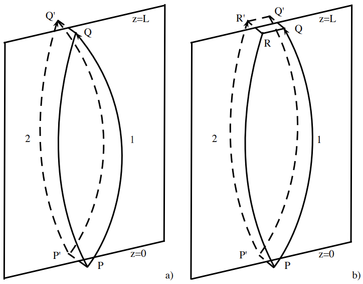
We first review the argument by Cowley et al. (1997), which is based on force-free MHD. For the purpose of showing a contradiction, they assume that a singular current sheet exists, as shown in Fig. A.1a. On the top of, yet infinitesimally close to the sheet, a magnetic field line starting from a point $P$ at $z = 0$ connects to a point $Q$ at $z = L$. Label this field line 1. On the bottom of the sheet, another field line 2 connects a point $P^{\prime}$ which is infinitesimally close to $P$, to a point $Q^{\prime}$ at $z = L$. With the footpoint motions assumed to be smooth, $Q^{\prime}$ must be infinitesimally close to $Q$ as well.
我们首先回顾 Cowley 等人(1997)的论点,该论点基于无力 MHD。为了显示矛盾,他们假设存在一个奇异电流片,如图 A.1a 所示。在片的顶部,但与片无限接近,从 $z = 0$ 处的点 $P$ 开始的一条磁力线连接到 $z = L$ 处的点 $Q$。将这条磁力线标记为 1。在片的底部,另一条磁力线 2 将一个与 $P$ 无限接近的点 $P^{\prime}$ 连接到 $z = L$ 处的点 $Q^{\prime}$。假设脚点运动是光滑的,那么 $Q^{\prime}$ 也必须与 $Q$ 无限接近。
Figure A.1: Illustrations for (a) a variant of van Ballegooijen’s argument by Cowley et al. (1997) and (b) our counter argument to it with a finite shear in the magnetic field properly considered.
图 A.1:图示(a)Cowley 等人(1997)对 van Ballegooijen 论点的变体,(b)我们对其的反驳,适当考虑了磁场中的有限剪切。
In a force-free equilibrium, the current density is parallel to the magnetic field, so that the current flows entirely along the current sheet and never leaves it (Cowley et al., 1997). Therefore, we have $\oint\mathbf{B}\cdot\mathrm{d}\mathbf{l}=0$ for any loop that lies on top or on the bottom of the sheet. For the path integral around the closed loop on the top of the sheet extending from $P$ to $Q$ along 1 and from $Q$ to $P$ along 2, as shown by the solid curves in Fig. A.1a, we have
$$ \oint\mathbf{B}\cdot\mathrm{d}\mathbf{l} = \int_{1}B_{1}(l)\mathrm{d}l - \int_{2}B_{1}(l)\cdot\mathbf{b}_{2}(l)\mathrm{d}l = 0. $$
Similarly, the path on the bottom of the sheet extending from $P^{\prime}$ to $Q^{\prime}$ along 2 and back to $P^{\prime}$ along 1, as shown by the dashed curves in Fig. A.1a, yields
$$ \oint\mathbf{B}\cdot\mathrm{d}\mathbf{l} = \int_{2}B_{2}(l)\mathrm{d}l - \int_{1}\mathbf{B}{2}(l)\cdot\mathbf{b}{1}(l)\mathrm{d}l = 0. $$
Here $\mathbf{B}_1$ and $\mathbf{B}_2$ are the magnetic fields on the top and the bottom of the sheet, while $\mathbf{b}_1$ and $\mathbf{b}_2$ are the corresponding unit vectors, respectively.
在无力平衡中,电流密度与磁场平行,因此电流完全沿着电流片流动,永远不会离开它(Cowley 等人,1997)。因此,对于任何位于片顶部或底部的环路,我们都有 $\oint\mathbf{B}\cdot\mathrm{d}\mathbf{l}=0$。对于沿 1 从 $P$ 到 $Q$ 沿 2 从 $Q$ 到 $P$ 的闭合环路上的路径积分,如图 A.1a 中的实线曲线所示,我们有
$$ \oint\mathbf{B}\cdot\mathrm{d}\mathbf{l} = \int_{1}B_{1}(l)\mathrm{d}l - \int_{2}B_{1}(l)\cdot\mathbf{b}_{2}(l)\mathrm{d}l = 0. $$
类似地,沿 2 从 $P^{\prime}$ 到 $Q^{\prime}$ 并沿 1 返回到 $P^{\prime}$ 的片底路径,如图 A.1a 中的虚线曲线所示,产生
$$ \oint\mathbf{B}\cdot\mathrm{d}\mathbf{l} = \int_{2}B_{2}(l)\mathrm{d}l - \int_{1}\mathbf{B}_{2}(l)\cdot\mathbf{b}_{1}(l)\mathrm{d}l = 0. $$
这里 $\mathbf{B}_1$ 和 $\mathbf{B}_2$ 分别是片的顶部和底部的磁场,而 $\mathbf{b}_1$ 和 $\mathbf{b}_2$ 分别是相应的单位向量。
The magnitude of the magnetic field must be continuous across the current sheet, that is, $B_1(l) = B_2(l) = B(l)$ (Cowley et al., 1997). We combine Eqs. (A.1) and (A.2) to obtain
$$ \int_{1+2}B(l)[1 - \mathbf{b}_{2}\cdot\mathbf{b}_{1}]\mathrm{d}l = 0. $$
This requires the unit vectors b1 and b2 to coincide, which means that the current sheet has no net current, contradicting the assumption of the singular current sheet.
磁场的大小必须在电流片上连续,即 $B_1(l) = B_2(l) = B(l)$(Cowley 等人,1997)。我们结合方程(A.1)和(A.2)得到
$$ \int_{1+2}B(l)[1 - \mathbf{b}_{2}\cdot\mathbf{b}_{1}]\mathrm{d}l = 0. $$
这要求单位向量 b1 和 b2 重合,这意味着电流片没有净电流,与奇异电流片的假设相矛盾。
Ng & Bhattacharjee (1998) remarked that the argument given above relies strongly on the assumptions regarding the geometry of the current sheet. They demonstrated that the argument fails for a current sheet with a geometry less trivial than the simple one shown in Fig. A.1a. Nonetheless, in this appendix, we show that even with such a simple geometry assumed, the above argument by Cowley et al. (1997) still does not stand.
Ng & Bhattacharjee(1998)指出,上述论点在很大程度上依赖于关于电流片几何形状的假设。他们证明了对于几何形状比图 A.1a 所示的简单几何形状更复杂的电流片,该论点是无效的。尽管如此,在本附录中,我们表明即使假设了如此简单的几何形状,Cowley 等人(1997)的上述论点仍然难以立足。
A crucial assumption implied in the above argument is that the footpoints of field line 2, $P^{\prime}$ and $Q^{\prime}$, are the mirror images of the footpoints of field line 1, $P$ and $Q$, with regard to the current sheet. That is, $PP^{\prime}$ and $QQ^{\prime}$ are both orthogonal to the current sheet. This is almost always not true. More generally, the shear in the footpoint motions, or equivalently, the magnetic field, would induce separations tangentially along the sheet as well. The linetied HKT problem considered in Chap. 4, among many others, is exactly a case of this kind.
在上述论点中隐含的一个关键假设是,磁力线 2 的脚点 $P^{\prime}$ 和 $Q^{\prime}$ 是磁力线 1 的脚点 $P$ 和 $Q$ 关于电流片的镜像。也就是说,$PP^{\prime}$ 和 $QQ^{\prime}$ 都垂直于电流片。这几乎总是不成立的。更一般地说,脚点运动中的剪切,或者等效地,在磁场中,也会沿着片面切向引起分离。第 4 章中考虑的线系 HKT 问题,以及许多其他问题,正是这种情况。
We treat the effect of the finite shear more carefully in Fig. A.1b. On the top of the sheet, the magnetic field line 1 still connects $P$ to $Q$. On the bottom of the sheet, we now choose $P^{\prime}$ to be the mirror image of $P$ with regard to the sheet. The field line 2 starting from $P^{\prime}$ connects to $R^{\prime}$ at $z = L$, which is not necessarily the mirror image of $Q$. Instead, we take $R$ and $Q^{\prime}$ to be the mirror images of $R^{\prime}$ and $Q$, respectively. Assuming $PP^{\prime}\sim QQ^{\prime}\sim RR^{\prime}\sim\epsilon$, which is infinitely small, we have $RQ\sim R^{\prime}Q^{\prime}\sim \epsilon s$, where $s$ stands for the finite shear across the sheet. When $\epsilon\rightarrow 0$, $R^{\prime}$ and $Q$ still coincide. However, as we shall show next, properly accounting for the finite shear $s$ can make a substantial difference.
我们在图 A.1b 中更仔细地处理有限剪切的影响。在片的顶部,磁力线 1 仍然将 $P$ 连接到 $Q$。在片的底部,我们现在选择 $P^{\prime}$ 作为 $P$ 关于片的镜像。从 $P^{\prime}$ 开始的磁力线 2 连接到 $z = L$ 处的 $R^{\prime}$,它不一定是 $Q$ 的镜像。相反,我们取 $R$ 和 $Q^{\prime}$ 分别为 $R^{\prime}$ 和 $Q$ 的镜像。假设 $PP^{\prime}\sim QQ^{\prime}\sim RR^{\prime}\sim\epsilon$,这是无限小的,我们有 $RQ\sim R^{\prime}Q^{\prime}\sim \epsilon s$,其中 $s$ 代表跨越片面的有限剪切。当 $\epsilon\rightarrow 0$ 时,$R^{\prime}$ 和 $Q$ 仍然重合。然而,正如我们接下来将展示的那样,正确考虑有限剪切 $s$ 可以产生实质性的差异。
For the path integral on the top of the sheet, along the solid curves in Fig. A.1b, Eq. (A.1) now becomes
$$ \oint\mathbf{B}\cdot\mathrm{d}\mathbf{l} = \int_{1}B_{1}(l)\mathrm{d}l + \int_{Q}^{R}\mathbf{B}\cdot\mathrm{d}\mathbf{l} - \int_{2}\mathbf{B}_{1}(l)\cdot\mathbf{b}_{2}(l)\mathrm{d}l = 0. $$
Similarly, along the path on the bottom of the sheet, as shown by the dashed curves in Fig. A.1b, Eq. (A.2) becomes
$$ \oint\mathbf{B}\cdot\mathrm{d}\mathbf{l} = \int_{2}B_{2}(l)\mathrm{d}l + \int_{R^{\prime}}^{Q^{\prime}}\mathbf{B}\cdot\mathrm{d}\mathbf{l} - \int_{1}\mathbf{B}_{2}(l)\cdot\mathbf{b}_{1}(l)\mathrm{d}l = 0. $$
Again, combining Eqs. (A.4) and (A.5), Eq. (A.3) becomes
$$ \int_{1+2}B(l)[1-\mathbf{b}_{2}(l)\cdot\mathbf{b}_{1}(l)]\mathrm{d}l = \int_{R}^{Q}\mathbf{B}\cdot\mathrm{d}\mathbf{l} + \int_{Q^{\prime}}^{R^{\prime}}\mathbf{B}\cdot\mathrm{d}\mathbf{l}. $$
Since the magnetic field has no normal component across the current sheet, the RHS can be expressed as a loop integral along $R\rightarrow Q\rightarrow Q^{\prime}\rightarrow R^{\prime}\rightarrow R$,
$$ \int_{1+2}B(l)[1-\mathbf{b}_{2}(l)\cdot\mathbf{b}_{1}(l)]\mathrm{d}l = \oint_{\partial\Omega}\mathbf{B}\cdot\mathrm{d}\mathbf{l} = \int_{\Omega}\mathbf{j}\cdot\mathrm{d}\mathbf{S}. $$
Here $\Omega$ is the area enclosed by this loop at the top plane $z = L$. As $\epsilon\rightarrow 0$, $\Omega\rightarrow 0$, but the RHS of Eq. (A.7) can be finite if and only if $j_{z}$ contains a 2D delta function at $z = L$. Still, this means that it is possible that $\mathbf{b}_{1}$ and $\mathbf{b}_{2}$ do not coincide, unlike what Cowley et al. (1997) claimed.
对于片顶部沿图 A.1b 中的实线曲线的路径积分,方程(A.1)现在变为
$$ \oint\mathbf{B}\cdot\mathrm{d}\mathbf{l} = \int_{1}B_{1}(l)\mathrm{d}l + \int_{Q}^{R}\mathbf{B}\cdot\mathrm{d}\mathbf{l} - \int_{2}\mathbf{B}_{1}(l)\cdot\mathbf{b}_{2}(l)\mathrm{d}l = 0. $$
类似地,沿着片底的路径,如图 A.1b 中的虚线曲线所示,方程(A.2)变为
$$ \oint\mathbf{B}\cdot\mathrm{d}\mathbf{l} = \int_{2}B_{2}(l)\mathrm{d}l + \int_{R^{\prime}}^{Q^{\prime}}\mathbf{B}\cdot\mathrm{d}\mathbf{l} - \int_{1}\mathbf{B}_{2}(l)\cdot\mathbf{b}_{1}(l)\mathrm{d}l = 0. $$
同样地,结合方程(A.4)和(A.5),方程(A.3)变为
$$ \int_{1+2}B(l)[1-\mathbf{b}_{2}(l)\cdot\mathbf{b}_{1}(l)]\mathrm{d}l = \int_{R}^{Q}\mathbf{B}\cdot\mathrm{d}\mathbf{l} + \int_{Q^{\prime}}^{R^{\prime}}\mathbf{B}\cdot\mathrm{d}\mathbf{l}. $$
由于磁场在电流片上没有法向分量,RHS 可以表示为沿 $R\rightarrow Q\rightarrow Q^{\prime}\rightarrow R^{\prime}\rightarrow R$ 的环路积分,
$$ \int_{1+2}B(l)[1-\mathbf{b}_{2}(l)\cdot\mathbf{b}_{1}(l)]\mathrm{d}l = \oint_{\partial\Omega}\mathbf{B}\cdot\mathrm{d}\mathbf{l} = \int_{\Omega}\mathbf{j}\cdot\mathrm{d}\mathbf{S}. $$
这里 $\Omega$ 是由该环路在顶面 $z = L$ 处包围的区域。当 $\epsilon\rightarrow 0$ 时,$\Omega\rightarrow 0$,但如果且仅当 $j_{z}$ 在 $z = L$ 处包含一个 2D delta 函数时,方程(A.7)的 RHS 可以是有限的。尽管如此,这意味着 $\mathbf{b}_{1}$ 和 $\mathbf{b}_{2}$ 不一定重合,这与 Cowley 等人(1997)的说法不同。
We emphasize that our argument in this appendix does not confirm the conjecture by Parker (1972). We merely show that the argument due to Cowley et al. (1997) that allegedly disproved Parker’s conjecture, which is a variant of that by van Ballegooijen (1985), does not really stand, and hence the Parker problem is still open.
我们强调,本附录中的论点并不证实 Parker(1972)的猜想。我们只是表明,Cowley 等人(1997)提出的据称反驳 Parker 猜想的论点,这是 van Ballegooijen(1985)论点的一个变体,实际上并不成立,因此 Parker 问题仍然是开放的。
In addition, the fact that $j_{z}$ needs to contain a 2D delta function at the footpoints in order for the singularity to exist suggests that the term “current sheet” may not accurately describe the possible singular structure in 3D line-tied geometry. Therefore, in this thesis, we adopt the more general term of “current singularity” instead.
此外,为了使奇点存在,$j_{z}$ 需要在脚点处包含一个 2D delta 函数,这表明 "电流片" 一词可能无法准确描述 3D 线系几何中可能的奇异结构。因此,在本论文中,我们采用更通用的“电流奇点”一词。
Appendix B: Numerical schemes
In this appendix, the update schemes of our variational integrators for ideal MHD in cartesian coordinates in 1D, 2D, and 3D are presented, respectively. In 2D and 3D, the schemes are derived on unstructured simplicial complexes.
本附录分别介绍了一维、二维和三维笛卡尔坐标下理想 MHD 的变分积分器更新方案。在二维和三维中,这些方案是在非结构简并复合物上推导出来的。
B.1 1D scheme
When projected into 1D, mass density and pressure become 1-forms. As for the magnetic field, a guide field is allowed. Its effect is exactly equivalent to a pressure with $\gamma=2$, so it can be treated as such. The Lagrangian in Lagrangian labeling (2.7) becomes
$$ L[x] = \int\left[\frac{1}{2}\rho_{0}\dot{x}^{2}-\frac{p_{0}}{\gamma-1J^{\gamma-1}}\right]\mathrm{d}x_{0}, $$
with the Jacobian $J=-\partial x/\partial x_{0}$. And the Euler-Lagrange equation becomes
$$ \rho_{0}\ddot{x} + \frac{\partial}{\partial x_{0}}\left(\frac{p_{0}}{J^{\gamma}}\right) = 0 $$
当投影到一维时,质量密度和压力就变成了一维形式。至于磁场,允许有导磁场。它的效果完全等同于 $\gamma=2$ 的压力,因此可以这样处理。拉格朗日标注(2.7)中的拉格朗日成为
$$ L[x] = \int\left[\frac{1}{2}\rho_{0}\dot{x}^{2}-\frac{p_{0}}{\gamma-1J^{\gamma-1}}\right]\mathrm{d}x_{0}, $$
雅可比行列式 $J=-\partial x/\partial x_{0}$。欧拉-拉格朗日方程变为
$$ \rho_{0}\ddot{x} + \frac{\partial}{\partial x_{0}}\left(\frac{p_{0}}{J^{\gamma}}\right) = 0 $$
Next we will spatially discretize the Lagrangian above. First, the manifold is discretized into $N + 1$ grids $x_{i}(i=0,1,\cdots,N)$ together with $N$ line segments $(x_{i},x_{i+1})$, where $x_{i}$ and $x_{i+1}$ are the left and right end of the segment respectively. The discrete 1-forms $\rho_{i}$ and $p_{i}$ are real numbers assigned to these segments. The initial grid size $x_{i+1}-x_{i}$ is denoted by a positive constant $h_{i}$ . In this case, the Jacobian becomes $J_{i} = (x_{i+1} − x_{i})/h_{i}$ . The kinetic energy term is a product of discrete mass densities on the line segments and the square of the velocities on the grids, and we choose to average the latter when multiplying. The spatially discretized Lagrangian is therefore
$$ L_{d}(x_{i},\dot{x}_{i}) = \sum_{i}\left[\frac{1}{2}\rho_{i}\frac{\dot{x}_{i}^{2}+\dot{x}_{i+1}^{2}}{2} - \frac{p_{i}}{(\gamma-1)J_{i}^{\gamma-1}}\right] = \sum_{i}\frac{1}{2}M_{i}\dot{x}_{i}^{2} - W(x_{i}) $$
where the subscript 0 on the initial conditions $\rho_{0i}$ and $p_{0i}$ are dropped for convenience, and $M_{i} = (\rho_{i-1} + \rho_{i})/2$ is the effective mass of the $i$th vertex. Note that $\rho_{i}$, $p_{i}$, and $M_{i}$ are all constants. This Lagrangian has the form of a many-body Lagrangian, and the consequent Euler-Lagrange equation has the form of a Newton's equation
$$ M_{i}\ddot{x}_{i} = -\frac{\partial W}{\partial x_{i}} = \frac{p_{i-1}/h_{i-1}}{(J_{i-1})^{\gamma}} - \frac{p_{i}/h_{i}}{(J_{i})^{\gamma}} = F_{i}(x_{i},x_{i\pm 1}) $$
接下来我们将对上述拉格朗日进行空间离散化。首先,将流形离散化为 $N + 1$ 个网格 $x_{i}(i=0,1,\cdots,N)$ 以及 $N$ 条线段 $(x_{i},x_{i+1})$,其中 $x_{i}$ 和 $x_{i+1}$ 分别是线段的左端和右端。离散一维形式 $\rho_{i}$ 和 $p_{i}$ 是分配给这些线段的实数。初始网格大小 $x_{i+1}-x_{i}$ 用一个正常数 $h_{i}$ 表示。在这种情况下,雅可比行列式变为 $J_{i} = (x_{i+1} − x_{i})/h_{i}$。动能项是线段上离散质量密度与网格上速度平方的乘积,我们选择在相乘时对后者进行平均。因此,空间离散化的拉格朗日为
$$ L_{d}(x_{i},\dot{x}_{i}) = \sum_{i}\left[\frac{1}{2}\rho_{i}\frac{\dot{x}_{i}^{2}+\dot{x}_{i+1}^{2}}{2} - \frac{p_{i}}{(\gamma-1)J_{i}^{\gamma-1}}\right] = \sum_{i}\frac{1}{2}M_{i}\dot{x}_{i}^{2} - W(x_{i}) $$
其中为了方便起见,初始条件 $\rho_{0i}$ 和 $p_{0i}$ 上的下标 0 被省略,$M_{i} = (\rho_{i-1} + \rho_{i})/2$ 是第 $i$ 个顶点的有效质量。注意,$\rho_{i}$、$p_{i}$ 和 $M_{i}$ 都是常数。这个拉格朗日具有多体拉格朗日的形式,因此随之而来的欧拉-拉格朗日方程具有牛顿方程的形式
$$ M_{i}\ddot{x}_{i} = -\frac{\partial W}{\partial x_{i}} = \frac{p_{i-1}/h_{i-1}}{(J_{i-1})^{\gamma}} - \frac{p_{i}/h_{i}}{(J_{i})^{\gamma}} = F_{i}(x_{i},x_{i\pm 1}) $$
For temporal discretization, we refer to Sec. 2.3. Boundary conditions can be introduced as holonomic constraints. For instance, one can choose periodic boundary condition with $x_{N} = x_{0} + L$, or ideal walls where $x_{1} = 0$ and $x_{N} = L$. Here the domain size $L = \sum_{i=1}^{N}h_{i}$ The effective mass needs to be adjusted accordingly for the boundary vertices as well. For periodic boundaries we have $M_{0} = M_{N} = (\rho_{0} + \rho_{N−1})/2$, while for ideal walls $M_{0} = \rho_{0}/2$ and $M_{N} = \rho_{N−1}/2$.
对于时间离散化,我们参考第 2.3 节。边界条件可以作为整体约束引入。例如,可以选择周期性边界条件 $x_{N} = x_{0} + L$,或者理想墙壁 $x_{1} = 0$ 和 $x_{N} = L$。这里的域大小 $L = \sum_{i=1}^{N}h_{i}$。边界顶点的有效质量也需要相应调整。对于周期性边界,我们有 $M_{0} = M_{N} = (\rho_{0} + \rho_{N−1})/2$,而对于理想墙壁 $M_{0} = \rho_{0}/2$ 和 $M_{N} = \rho_{N−1}/2$。
B.2 2D scheme
When projected into 2D, mass density and pressure become 2-forms. The effective mass of a vertex $\sigma_{0}$ becomes $M(\sigma_{0}^{0}) = \sum_{\sigma_{0}^{2}>\sigma_{0}^{0}}\langle \rho_{0},\sigma_{0}^{2}\rangle/3$. The guide field can effectively be treated as a magnetic pressure with $\gamma = 2$. Hence we only need to consider the in-plane magnetic field, which becomes a 1-form. The Lagrangian and the Euler-Lagrange equation are basically the same as Eqs. (2.7) and (2.8), except in lower dimension. Note that the 1D derivation above is based on a structure grid, since any grid is naturally structured in 1D. But in 2D the mesh becomes genuinely unstructured, so we need to adopt a more abstract terminology. As can be seen from Sec. 2.3, one only needs to calculate the discrete potential energy $W$ of an arbitrary volume simplex, and then derive its force on its $i$th vertex. Then one can iterate over all the volume simplices and calculate the total force on each vertex.
当投影到二维时,质量密度和压力变成二维形式。顶点 $\sigma_{0}$ 的有效质量变为 $M(\sigma_{0}^{0}) = \sum_{\sigma_{0}^{2}>\sigma_{0}^{0}}\langle \rho_{0},\sigma_{0}^{2}\rangle/3$。导磁场可以有效地视为 $\gamma = 2$ 的磁压力。因此,我们只需要考虑面内磁场,它变成了一维形式。拉格朗日和欧拉-拉格朗日方程基本上与方程(2.7)和(2.8)相同,只是维度较低。请注意,上述一维推导是基于结构化网格的,因为在一维中任何网格自然都是结构化的。但在二维中,网格变得真正非结构化,因此我们需要采用更抽象的术语。正如第 2.3 节所示,人们只需要计算任意体积单纯形的离散势能 $W$,然后推导其对第 $i$ 个顶点的力。然后可以遍历所有体积单纯形并计算每个顶点上的总力。
Following from Eq. (2.17), the potential energy for a 2-simplex $(0, 1, 2)$, namely a triangle, reads
$$ W = \frac{p}{(\gamma-1)(S/S_{0})^{\gamma-1}} + \frac{1}{8S}\sum_{i=0}^{L}B_{i}^{2}I_{i}, $$
where $p$ is the initial pressure, $B_{i}$ is the initial magnetic field evaluated on the edge opposite to vertex $i$, and the area
$$ S = [(x_{i+1}-x_{i})(y_{i+2}-y_{i}) - (x_{i+2}-x_{i})(x_{i+2}-x_{i})]/2. $$
Here $i = 0, 1, 2$, and operation mod 3 is implied on the vertex indices (subscripts) $i + 1$ and $i + 2$. $S_{0}$ is the initial area, and $p$, $B_{i}$ and $S_{0}$ are all constants. The inner product with respect to vertex $i$ reads
$$ I_{i} = (x_{i+1} - x_{i})(x_{i+2}-x_{i}) + (y_{i+1} - y_{i})(y_{i+2}-y_{i}). $$
Then, taking the derivative of $W$ then leads to the force on vertex $j$,
$$ \begin{align*} -\frac{\partial W}{\partial x_{j}} = & \left[\frac{p/S_{0}}{2(S/S_{0})^{\gamma}} + \frac{1}{16A^{2}}\sum_{i=0}^{2}B_{i}^{2}I_{i}\right](y_{j+1} - y_{j+2})\\ +& [(B_{j+2}^{2}-B_{j+1}^{2})(x_{j+1}-x_{j+2})+B_{j}^{2}(2x_{j}-x_{j+1}-x_{j+2})]/(8S),\\ -\frac{\partial W}{\partial y_{j}} = & -\left[\frac{p/S_{0}}{2(S/S_{0})^{\gamma}} + \frac{1}{16A^{2}}\sum_{i=0}^{2}B_{i}^{2}I_{i}\right](x_{j+2} - x_{j+1})\\ +& [(B_{j+2}^{2}-B_{j+1}^{2})(y_{j+1}-y_{j+2})+B_{j}^{2}(2y_{j}-y_{j+1}-y_{j+2})]/(8S). \end{align*} $$
Again, j = 0, 1, 2, and the subscripts $j + 1$ and $j + 2$ are subject to operation mod 3.
同样地,沿用方程(2.17),2-单纯形 $(0, 1, 2)$,即三角形的势能为
$$ W = \frac{p}{(\gamma-1)(S/S_{0})^{\gamma-1}} + \frac{1}{8S}\sum_{i=0}^{L}B_{i}^{2}I_{i}, $$
其中 $p$ 是初始压力,$B_{i}$ 是在顶点 $i$ 对边上评估的初始磁场,面积为
$$ S = [(x_{i+1}-x_{i})(y_{i+2}-y_{i}) - (x_{i+2}-x_{i})(x_{i+2}-x_{i})]/2. $$
这里 $i = 0, 1, 2$,并且对顶点索引(下标)$i + 1$ 和 $i + 2$ 隐含模 3 运算。$S_{0}$ 是初始面积,$p$、$B_{i}$ 和 $S_{0}$ 都是常数。关于顶点 $i$ 的内积为
$$ I_{i} = (x_{i+1} - x_{i})(x_{i+2}-x_{i}) + (y_{i+1} - y_{i})(y_{i+2}-y_{i}). $$
然后,对 $W$ 求导得到顶点 $j$ 上的力,
$$ \begin{align*} -\frac{\partial W}{\partial x_{j}} = & \left[\frac{p/S_{0}}{2(S/S_{0})^{\gamma}} + \frac{1}{16A^{2}}\sum_{i=0}^{2}B_{i}^{2}I_{i}\right](y_{j+1} - y_{j+2})\\ +& [(B_{j+2}^{2}-B_{j+1}^{2})(x_{j+1}-x_{j+2})+B_{j}^{2}(2x_{j}-x_{j+1}-x_{j+2})]/(8S),\\ -\frac{\partial W}{\partial y_{j}} = & -\left[\frac{p/S_{0}}{2(S/S_{0})^{\gamma}} + \frac{1}{16A^{2}}\sum_{i=0}^{2}B_{i}^{2}I_{i}\right](x_{j+2} - x_{j+1})\\ +& [(B_{j+2}^{2}-B_{j+1}^{2})(y_{j+1}-y_{j+2})+B_{j}^{2}(2y_{j}-y_{j+1}-y_{j+2})]/(8S). \end{align*} $$
同样地,j = 0, 1, 2,并且下标 $j + 1$ 和 $j + 2$ 受模 3 运算影响。
Boundary conditions can again be introduced as holonomic constraints. Besides periodic boundaries, there can also be ideal walls and no-slip boundaries. For ideal walls, the vertices on the boundaries are allowed to move tangentially along, but not normally to them. For no-slip boundaries, the vertices on the boundaries do not move.
边界条件同样可以作为整体约束引入。除了周期性边界外,还有理想墙壁和无滑移边界。对于理想墙壁,边界上的顶点允许沿着边界切向移动,但不能垂直于边界移动。对于无滑移边界,边界上的顶点不移动。
B.3 3D scheme
For 3D MHD, we carry out the same procedure as in 2D. Following from Eq. (2.17), the potential energy for a 3-simplex (0, 1, 2, 3), a tetrahedron, reads
$$ W = \frac{p}{(\gamma-1)(V/V_{0})^{\gamma-1}} + \frac{1}{12V}\sum_{i=0}^{3}B_{i}^{2}\beta_{i}/S_{i}^{2}, $$
where $p$ is the initial pressure, $B_{i}$ is the initial magnetic field evaluated on the face opposite to vertex $i$. $V$ is the volume of the tetrahedron, while $V_{0}$ is its initial value. $p$, $B_i$ and $V_0$ are constants. $\beta_{i}$ is the barycentric coordinate with regard to vertex,
$$ \beta_{i} = \sum_{k=0}^{2}l_{i,i+1+k}^{2}l_{i+1+(k+1),i+1+(k+2)}^{2}I_{i,k} - 2l_{i+2,i+3}l_{i+1,i+3}^{2}l_{i+2,i+1}^{2}. $$
Here the squared length of the edge $(i, j)$ is
$$ l_{i,j}^{2} = (x_{i}-x_{j})^{2} + (y_{i}-y_{j})^{2} + (z_{i}-z_{j})^{2}, $$
while $I_{i,k}$ denotes the doubled inner product with regard to vertex $i + 1 + k$ in the face opposite to vertex $i$,
$$ I_{i,k} = l_{i+1+k,i+1+(k+1)}^{2} + l_{i+1+k,i+1+(k+2)}^{2} - l_{i+1+(k+2),i+1+(k+1)}^{2} $$
Note that here $(k + 1)$, $(k + 2)$ are subject to operation mod 3, and all the vertex indices (subscripts), such as $i + 1 + k$, $i + 1 + (k + 1)$, and $i + 1 + (k + 2)$ are subject to operation mod 4. The same applies to the rest of this section. Similarly, the sixteen-timed squared area of the face opposite to vertex $i$ is given by
$$ S_{i}^{2} = \sum_{k=0}^{2}l_{i+1+(k+1),i+1+(k+2)}I_{i,k}. $$
对于三维 MHD,我们执行与二维中相同的过程。沿用方程(2.17),3-单纯形 (0, 1, 2, 3),即四面体的势能为
$$ W = \frac{p}{(\gamma-1)(V/V_{0})^{\gamma-1}} + \frac{1}{12V}\sum_{i=0}^{3}B_{i}^{2}\beta_{i}/S_{i}^{2}, $$
其中 $p$ 是初始压力,$B_{i}$ 是在顶点 $i$ 对面的面上评估的初始磁场。$V$ 是四面体的体积,而 $V_{0}$ 是其初始值。$p$、$B_i$ 和 $V_0$ 是常数。$\beta_{i}$ 是关于顶点的重心坐标,
$$ \beta_{i} = \sum_{k=0}^{2}l_{i,i+1+k}^{2}l_{i+1+(k+1),i+1+(k+2)}^{2}I_{i,k} - 2l_{i+2,i+3}l_{i+1,i+3}^{2}l_{i+2,i+1}^{2}. $$
这里边 $(i, j)$ 的平方长度为
$$ l_{i,j}^{2} = (x_{i}-x_{j})^{2} + (y_{i}-y_{j})^{2} + (z_{i}-z_{j})^{2}, $$
而 $I_{i,k}$ 表示关于顶点 $i + 1 + k$ 的面 $i$ 对面的二倍内积,
$$ I_{i,k} = l_{i+1+k,i+1+(k+1)}^{2} + l_{i+1+k,i+1+(k+2)}^{2} - l_{i+1+(k+2),i+1+(k+1)}^{2} $$
请注意,这里 $(k + 1)$、$(k + 2)$ 受模 3 运算影响,所有顶点索引(下标),例如 $i + 1 + k$、$i + 1 + (k + 1)$ 和 $i + 1 + (k + 2)$ 都受模 4 运算影响。本节的其余部分也是如此。同样地,顶点 $i$ 对面的面的十六倍平方面积由下式给出
$$ S_{i}^{2} = \sum_{k=0}^{2}l_{i+1+(k+1),i+1+(k+2)}I_{i,k}. $$
Again, the force follows from taking the derivative of the potential energy,
$$ -\frac{\partial W}{\partial x_{j}} = \left[\frac{p/V_{0}}{(V/V_{0})^{\gamma}} + \frac{1}{12V^{2}}\sum_{i=0}^{3}B_{i}^{2}\beta_{i}/S_{i}^{2}\right]\frac{\partial V}{\partial x_{j}} - \frac{1}{12V}\sum_{i=0}^{3}\frac{B_{i}^{2}}{S_{i}^{2}}\left(\frac{\partial \beta_{i}}{\partial x_{j}}-\frac{\beta_{i}}{S_{i}^{2}}\frac{\partial S_{i}^{2}}{\partial x_{j}}\right). $$
Here we only show the $x$ component, as the $y$ and $z$ components can be obtained by shuffling $x$, $y$, and $z$. Note that
$$ \frac{\partial V}{\partial x_{j}} = \frac{(-1)^{j-1}}{6}\sum_{k=0}^{2}y_{j+1+k}[z_{j+1+(k+1)}-z_{j+1+(k+2)}], $$
and the volume can be calculated by
$$ V = \sum_{j=0}^{3}x_{j}\frac{\partial V}{\partial x_{j}} $$
When calculating $\partial S_{i}^{2}/\partial x_{j}$ and $\partial\beta_{i}/\partial x_{j}$, one needs to differentiate between when $i = j$ and when $i\neq j$. For the doubled area, $\partial S_{i}^{2}/\partial x_{i}$, while
$$ \partial S_{i}^{2}/\partial x_{i+1+k} = 4[x_{i+1+k} - x_{i+1+(k+1)}]I_{i,(k+2)} + 4[x_{i+1+k} - x_{i+1+(k+2)}]I_{i,(k+1)}, $$
for $k = 0, 1, 2$. Finally, the derivatives for the barycentric coordinates read
$$ \begin{align*} \frac{\partial\beta_{i}}{\partial x_{i}} &= \sum_{k=0}^{2}2[x_{i} - x_{i+1+k}]l_{i+1+(k+1), i+1+(k+2)}I_{i,k},\\ \frac{\partial\beta_{i}}{\partial x_{i+1+k}} &= 2[x_{i+1+k} - x_{i+1+(k+1)}]\cdots \end{align*} $$